Comparison of ERA5 and IMD Daily Temperature Extremes Across Maharashtra (2024)#
In this notebook, we analyze and compare daily temperature extremes patterns across Maharashtra using two key datasets:
ERA5: Climate reanalysis data from ECMWF
IMD: Gridded daily temperature extremes from the Indian Meteorological Department
We focus on:
Harmonizing ERA5 and IMD temperature data
Evaluating the correlation between ERA5 and IMD temperature extremes at each grid point
Visualizing the spatial pattern of Pearson correlations to assess agreement between datasets
We use:
varunayanfor extracting ERA5 hourly minimum and maximum temperaturesimdlibfor accessing IMD daily tmin and tmax data
This study provides insights into how well ERA5 captures regional temperature extremes in Maharashtra compared to IMD observations, which could be important for validating ERA5 use in climate research and studies for Maharashtra.
Step 1: Extract ERA5 Temperature Extremes Data for Maharashtra#
We use varunayan to download hourly minimum and maximum temperature (mn2t and mx2t) from the ERA5 climate reanalysis dataset for the Maharashtra region, covering the year 2024.
North: 21.5°, South: 15.5°, East: 80.5°, West: 72.5°
Resolution: 1°
Frequency: hourly
Units: Kelvin
We will be using the raw data acquired using varunayan for this analysis.
import varunayan

varunayan.era5ify_bbox(
    request_id='min_max_temp_maha_2020',
    variables=['maximum_2m_temperature_since_previous_post_processing', 'minimum_2m_temperature_since_previous_post_processing'],
    start_date='2020-1-1',
    end_date='2020-12-31',
    north=21.5,
    south=15.5,
    east=80.5,
    west=72.5,
    resolution=1,
)
============================================================
STARTING ERA5 SINGLE LEVEL PROCESSING
============================================================
Request ID: min_max_temp_maha_2020
Variables: ['maximum_2m_temperature_since_previous_post_processing', 'minimum_2m_temperature_since_previous_post_processing']
Date Range: 2020-01-01 to 2020-12-31
Frequency: hourly
Resolution: 1°
Saving files to output directory: min_max_temp_maha_2020_output
  Saved final data to: min_max_temp_maha_2020_output\min_max_temp_maha_2020_hourly_data.csv
  Saved unique coordinates to: min_max_temp_maha_2020_output\min_max_temp_maha_2020_unique_latlongs.csv
  Saved raw data to: min_max_temp_maha_2020_output\min_max_temp_maha_2020_raw_data.csv

============================================================
PROCESSING COMPLETE
============================================================

RESULTS SUMMARY:
----------------------------------------
Variables processed: 2
Time period:         2020-01-01 to 2020-12-31
Final output shape:  (8784, 7)
Total complete processing time: 2865.08 seconds

First 5 rows of aggregated data:
         mx2t        mn2t        date  year  month  day  hour
0  299.386475  286.384277  2020-01-01  2020      1    1     0
1  299.424072  286.346191  2020-01-01  2020      1    1     1
2  299.484619  286.520264  2020-01-01  2020      1    1     2
3  299.594971  286.739990  2020-01-01  2020      1    1     3
4  299.720703  288.402100  2020-01-01  2020      1    1     4

============================================================
ERA5 SINGLE LEVEL PROCESSING COMPLETED SUCCESSFULLY
============================================================
| mx2t | mn2t | date | year | month | day | hour | |
|---|---|---|---|---|---|---|---|
| 0 | 299.386475 | 286.384277 | 2020-01-01 | 2020 | 1 | 1 | 0 |
| 1 | 299.424072 | 286.346191 | 2020-01-01 | 2020 | 1 | 1 | 1 |
| 2 | 299.484619 | 286.520264 | 2020-01-01 | 2020 | 1 | 1 | 2 |
| 3 | 299.594971 | 286.739990 | 2020-01-01 | 2020 | 1 | 1 | 3 |
| 4 | 299.720703 | 288.402100 | 2020-01-01 | 2020 | 1 | 1 | 4 |
| ... | ... | ... | ... | ... | ... | ... | ... |
| 8779 | 301.058594 | 288.187988 | 2020-12-31 | 2020 | 12 | 31 | 19 |
| 8780 | 301.026367 | 287.927979 | 2020-12-31 | 2020 | 12 | 31 | 20 |
| 8781 | 300.906494 | 287.406494 | 2020-12-31 | 2020 | 12 | 31 | 21 |
| 8782 | 300.800781 | 286.872314 | 2020-12-31 | 2020 | 12 | 31 | 22 |
| 8783 | 300.804199 | 286.522705 | 2020-12-31 | 2020 | 12 | 31 | 23 |
8784 rows × 7 columns
Step 2: Process ERA5 Temperature Extremes Data#
We process the downloaded ERA5 dataset to compute daily temperature extremes in Celsius.
Key steps:#
Convert from Kelvin to Celsius
Subtract 273.15 from
mx2tandmn2tvaluesFinal unit: °C
Aggregate to Daily Extremes (Per Grid Point)
Compute daily maximum (
mx2t) and minimum (mn2t) temperatures for each latitude–longitude point
The result is a dataframe (daily_era5_data) with the columns:
latitude,longitude,date,mx2tandmn2t
import pandas as pd

df_raw_temp = pd.read_csv('min_max_temp_maha_2020_output/min_max_temp_maha_2020_raw_data.csv')
df_raw_temp['date'] = pd.to_datetime(df_raw_temp['date'])
df_raw_temp['mx2t'] = df_raw_temp['mx2t'] - 273.15
df_raw_temp['mn2t'] = df_raw_temp['mn2t'] - 273.15
df_daily_era = (
    df_raw_temp.groupby(["latitude", "longitude", "date"])
    .agg({
        "mx2t": "max",
        "mn2t": "min",
    })
    .reset_index()
)
Step 3: Extract IMD Gridded Temperature Data#
We use the imdlib package to download daily gridded IMD temperature extremes data over Maharashtra.
Variables:
'tmax'and'tmin'Grid resolution: 1°
Unit: °C
This dataset represents observed temperature extremes, derived from IMD’s high-quality station network and gridded for regional analysis. While the 1° resolution provides a broad spatial overview, it limits finer scale temperature analysis, a constraint in IMD’s open temperature dataset.
import imdlib as imd

start_yr = 2020
variable = 'tmax'
imd.get_data(variable, start_yr, fn_format='monthwise')

import numpy as np

data = imd.open_data(variable, start_yr, fn_format='monthwise')
ds = data.get_xarray()
df = ds.to_dataframe().reset_index()
df['tmax'] = df['tmax'].replace(-999.0, np.nan)

df_bbox_max = df[
    (df['lat'] >= 15) & (df['lat'] <= 22) &
    (df['lon'] >= 72) & (df['lon'] <= 81)
]

df_bbox_max.reset_index(drop=True, inplace=True)

df_bbox_max
Downloading: maxtemp for year 2020
Download Successful !!!
| time | lat | lon | tmax | |
|---|---|---|---|---|
| 0 | 2020-01-01 | 15.5 | 72.5 | 99.900002 |
| 1 | 2020-01-01 | 15.5 | 73.5 | 31.408098 |
| 2 | 2020-01-01 | 15.5 | 74.5 | 31.509253 |
| 3 | 2020-01-01 | 15.5 | 75.5 | 31.085457 |
| 4 | 2020-01-01 | 15.5 | 76.5 | 30.606255 |
| ... | ... | ... | ... | ... |
| 23053 | 2020-12-31 | 21.5 | 76.5 | 28.515602 |
| 23054 | 2020-12-31 | 21.5 | 77.5 | 27.787882 |
| 23055 | 2020-12-31 | 21.5 | 78.5 | 26.746124 |
| 23056 | 2020-12-31 | 21.5 | 79.5 | 26.715961 |
| 23057 | 2020-12-31 | 21.5 | 80.5 | 27.381311 |
23058 rows × 4 columns
import imdlib as imd

start_yr = 2020
variable = 'tmin'
imd.get_data(variable, start_yr, fn_format='monthwise')

import numpy as np

data = imd.open_data(variable, start_yr, fn_format='monthwise')
ds = data.get_xarray()
df = ds.to_dataframe().reset_index()
df['tmin'] = df['tmin'].replace(-999.0, np.nan)

df_bbox_min = df[
    (df['lat'] >= 15) & (df['lat'] <= 22) &
    (df['lon'] >= 72) & (df['lon'] <= 81)
]

df_bbox_min.reset_index(drop=True, inplace=True)

df_bbox_min
Downloading: mintemp for year 2020
Download Successful !!!
| time | lat | lon | tmin | |
|---|---|---|---|---|
| 0 | 2020-01-01 | 15.5 | 72.5 | 99.900002 |
| 1 | 2020-01-01 | 15.5 | 73.5 | 17.982029 |
| 2 | 2020-01-01 | 15.5 | 74.5 | 18.658150 |
| 3 | 2020-01-01 | 15.5 | 75.5 | 17.838404 |
| 4 | 2020-01-01 | 15.5 | 76.5 | 18.578913 |
| ... | ... | ... | ... | ... |
| 23053 | 2020-12-31 | 21.5 | 76.5 | 12.886724 |
| 23054 | 2020-12-31 | 21.5 | 77.5 | 12.003990 |
| 23055 | 2020-12-31 | 21.5 | 78.5 | 11.423929 |
| 23056 | 2020-12-31 | 21.5 | 79.5 | 10.512906 |
| 23057 | 2020-12-31 | 21.5 | 80.5 | 11.225183 |
23058 rows × 4 columns
Step 4: Merge ERA5 and IMD DataFrames and Compute Correlations#
In this step, we merge the three datasets:
ERA5 daily temperature extremes
IMD daily minimum temperature (
tmin)IMD daily maximum temperature (
tmax)
The merge is performed on the shared columns: date, latitude, and longitude.
After merging, we compute Pearson correlation coefficients between ERA5 and IMD temperature extremes to assess their agreement at each grid point.
df_bbox_max = df_bbox_max.rename(columns={'time': 'date', 'lat': 'latitude', 'lon': 'longitude'})
df_bbox_min = df_bbox_min.rename(columns={'time': 'date', 'lat': 'latitude', 'lon': 'longitude'})

# First merge max and min
df_bbox = pd.merge(df_bbox_max, df_bbox_min, on=['latitude', 'longitude', 'date'])

# Then merge with ERA5 data
df_merged = pd.merge(df_bbox, df_daily_era, on=['latitude', 'longitude', 'date'])
df_clean = df_merged[
    (df_merged['tmax'] != 99.900002) &
    (df_merged['tmin'] != 99.900002)
].copy()
from scipy.stats import pearsonr

def compute_corr(group):
    tmax_corr = pearsonr(group['tmax'], group['mx2t'])[0]
    tmin_corr = pearsonr(group['tmin'], group['mn2t'])[0]
    return pd.Series({'tmax_corr': tmax_corr, 'tmin_corr': tmin_corr})

correlations = df_clean.groupby(['latitude', 'longitude']).apply(compute_corr).reset_index()
C:\Users\Atharva Jagtap\AppData\Local\Temp\ipykernel_7744\3252918934.py:8: FutureWarning: DataFrameGroupBy.apply operated on the grouping columns. This behavior is deprecated, and in a future version of pandas the grouping columns will be excluded from the operation. Either pass `include_groups=False` to exclude the groupings or explicitly select the grouping columns after groupby to silence this warning.
  correlations = df_clean.groupby(['latitude', 'longitude']).apply(compute_corr).reset_index()
Step 5: Visualize Grid Point Correlations with Maharashtra Block Boundaries#
In this step, we create spatial visualizations of the Pearson correlation coefficients between ERA5 and IMD temperature extremes, computed at each grid point.
Plot Details:
Each grid point is color-coded based on the correlation value (using a colormap)
Separate plots may be generated for
tmaxandtmincorrelationsThe underlying map includes Maharashtra’s block-level administrative boundaries, overlaid using a GeoJSON file
This visualization helps assess the spatial consistency of ERA5 with IMD across different parts of Maharashtra and identifies regions with high or low agreement between datasets.
import pandas as pd
import geopandas as gpd
import matplotlib.pyplot as plt
import numpy as np

correlations[['tmax_corr', 'tmin_corr']] = correlations[['tmax_corr', 'tmin_corr']].fillna(0)

# Create GeoDataFrame
gdf = gpd.GeoDataFrame(
    correlations,
    geometry=gpd.points_from_xy(correlations['longitude'], correlations['latitude']),
    crs="EPSG:4326"
)

# Load Maharashtra blocks GeoJSON
maha = gpd.read_file("https://maharashtra-blocks-geojson.netlify.app/maharashtra_blocks.geojson")

# Shared color limits
vmin = min(gdf[['tmax_corr', 'tmin_corr']].min())
vmax = max(gdf[['tmax_corr', 'tmin_corr']].max())

# Plot
fig, ax = plt.subplots(1, 2, figsize=(14, 7), constrained_layout=True)

# Plot tmax_corr
maha.boundary.plot(ax=ax[0], color='black', linewidth=0.5)
sc1 = gdf.plot(
    ax=ax[0], column='tmax_corr', cmap='viridis', markersize=50,
    vmin=vmin, vmax=vmax, legend=True, legend_kwds={'label': 'Pearson R'}
)
ax[0].set_title('tmax (from IMD) vs mx2t (from ERA5)')
ax[0].set_xlabel('Longitude')
ax[0].set_ylabel('Latitude')

# Plot tmin_corr
maha.boundary.plot(ax=ax[1], color='black', linewidth=0.5)
sc2 = gdf.plot(
    ax=ax[1], column='tmin_corr', cmap='viridis', markersize=50,
    vmin=vmin, vmax=vmax, legend=True, legend_kwds={'label': 'Pearson R'}
)
ax[1].set_title('tmin (from IMD) vs mn2t (from ERA5)')
ax[1].set_xlabel('Longitude')
ax[1].set_ylabel('Latitude')

# Consistent aspect ratio
for a in ax:
    a.set_aspect('equal')

plt.show()
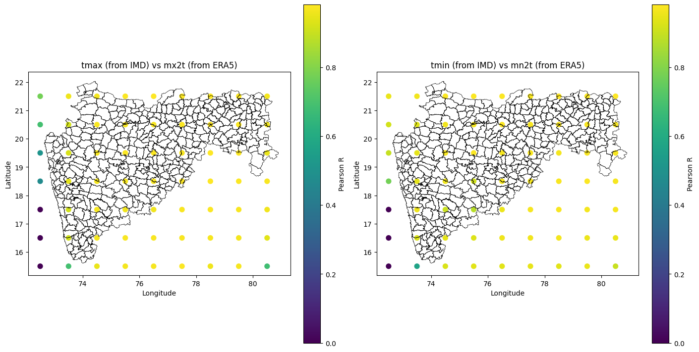
As we can see in the plot above, the correlation between the two datasets is strong over the mainland and weak over the Arabian Sea.
correlations.to_csv('correlation_maha_2020_tmax_tmin.csv', index=False)