Visualizing Climate Change in India#
In this vignette, we show how to use varunayan to easily extract annual average temperature data for India and visualize the temperature changes over the period from 1941 to 2024.
Step 1: Download Temperature Data for India#
We use varunayan.era5ify_geojson to download yearly average 2m temperature data for India, using a GeoJSON boundary file from a public URL.
import varunayan

df = varunayan.era5ify_geojson(
    request_id="temp_india_yearly",
    variables=["2m_temperature"],
    start_date="1941-1-1",
    end_date="2024-12-31",
    json_file="https://gist.githubusercontent.com/JaggeryArray/bf296307132e7d6127e28864c7bea5bf/raw/4bce03beea35d61a93007f54e52ba81f575a7feb/india.json",
    frequency="yearly",
)
============================================================
STARTING ERA5 SINGLE LEVEL PROCESSING
============================================================
Request ID: temp_india_yearly
Variables: ['2m_temperature']
Date Range: 1941-01-01 to 2024-12-31
Frequency: yearly
Resolution: 0.25°
GeoJSON File: C:\Users\ATHARV~1\AppData\Local\Temp\temp_india_yearly_temp_geojson.json


--- GeoJSON Mini Map ---

MINI MAP (68.18°W to 97.40°E, 7.97°S to 35.49°N):
┌─────────────────────────────────────────┐
│·········································│
│········■■■■■■■··························│
│··········■■■■■··························│
│·········■■■■■■■·························│
│·······■■■■■■■■■■························│
│····■■■■■■■■■■■■■■■■········■····■■■■■■■·│
│···■■■■■■■■■■■■■■■■■■■■■■■■■·■■■■■■■■····│
│····■■■■■■■■■■■■■■■■■■■■■■■■·····■■■■····│
│·■■■■■■■■■■■■■■■■■■■■■■■■■■■■···■■■······│
│··■■■■■■■■■■■■■■■■■■■■■■■■■■■············│
│·······■■■■■■■■■■■■■■■■■■■···············│
│·······■■■■■■■■■■■■■■■■··················│
│·······■■■■■■■■■■■■■·····················│
│········■■■■■■■■■························│
│·········■■■■■■■■························│
│··········■■■■■■■························│
│···········■■■■■·························│
│············■■■··························│
│·········································│
└─────────────────────────────────────────┘
 ■ = Inside the shape
 · = Outside the shape
Saving files to output directory: temp_india_yearly_output
  Saved final data to: temp_india_yearly_output\temp_india_yearly_yearly_data.csv
  Saved unique coordinates to: temp_india_yearly_output\temp_india_yearly_unique_latlongs.csv
  Saved raw data to: temp_india_yearly_output\temp_india_yearly_raw_data.csv

============================================================
PROCESSING COMPLETE
============================================================

RESULTS SUMMARY:
----------------------------------------
Variables processed: 1
Time period:         1941-01-01 to 2024-12-31
Final output shape:  (84, 2)
Total complete processing time: 447.03 seconds

First 5 rows of aggregated data:
          t2m  year
0  296.386200  1941
1  296.234344  1942
2  295.743408  1943
3  296.361176  1944
4  296.111603  1945

============================================================
ERA5 SINGLE LEVEL PROCESSING COMPLETED SUCCESSFULLY
============================================================
Step 2: Compute Deviation from Long-Term Mean#
We calculate the deviation of each year’s average temperature from the long-term mean. This helps us understand how each year compares to the overall average.
mean_t2m = df["t2m"].mean()

df["dev"] = df["t2m"] - mean_t2m

df.head()
| t2m | year | dev | |
|---|---|---|---|
| 0 | 296.386200 | 1941 | -0.202301 |
| 1 | 296.234344 | 1942 | -0.354156 |
| 2 | 295.743408 | 1943 | -0.845093 |
| 3 | 296.361176 | 1944 | -0.227325 |
| 4 | 296.111603 | 1945 | -0.476898 |
Step 3: Set Up Matplotlib Styling#
We configure Matplotlib to ensure consistent, high-resolution plots with a clean visual style. This setup improves readability, especially in documentation.
import matplotlib.cm as cm
import matplotlib.colors as mcolors
import matplotlib.pyplot as plt


def setup_matplotlib():
    plt.rcParams["figure.dpi"] = 300
    plt.rcParams["savefig.dpi"] = 300
    plt.rcParams["font.family"] = "sans-serif"
    plt.rcParams["font.sans-serif"] = ["Arial"]
    plt.rcParams["axes.labelweight"] = "normal"

    plt.rcParams["mathtext.fontset"] = "custom"
    plt.rcParams["mathtext.rm"] = "Arial"
    plt.rcParams["mathtext.it"] = "Arial:italic"
    plt.rcParams["mathtext.bf"] = "Arial:bold"


setup_matplotlib()
Step 4: Normalize Deviation Values#
We normalize the temperature deviation values so we can map them to a color scale for the bar chart.
norm = mcolors.Normalize(vmin=df["dev"].min(), vmax=df["dev"].max())
Step 5: Set Color Map#
We use the coolwarm color map to represent deviation: cool colors for below-average years and warm colors for above-average years.
cmap = plt.colormaps["coolwarm"]
colors = cmap(norm(df["dev"]))
Step 6: Plot Temperature Deviation Over Time#
We create a color-coded bar plot of yearly temperature deviations. A colorbar is added to indicate the scale of deviation from the mean.
fig, ax = plt.subplots(figsize=(14, 6))
bars = ax.bar(df["year"], df["dev"], color=colors)

sm = cm.ScalarMappable(cmap=cmap, norm=norm)
sm.set_array(df["dev"].values)

cbar = fig.colorbar(sm, ax=ax)
cbar.set_label("Deviation")

ax.set_xlabel("Year")
ax.set_ylabel("Deviation")
ax.set_title("Temperature change in India")

plt.tight_layout()
plt.show()
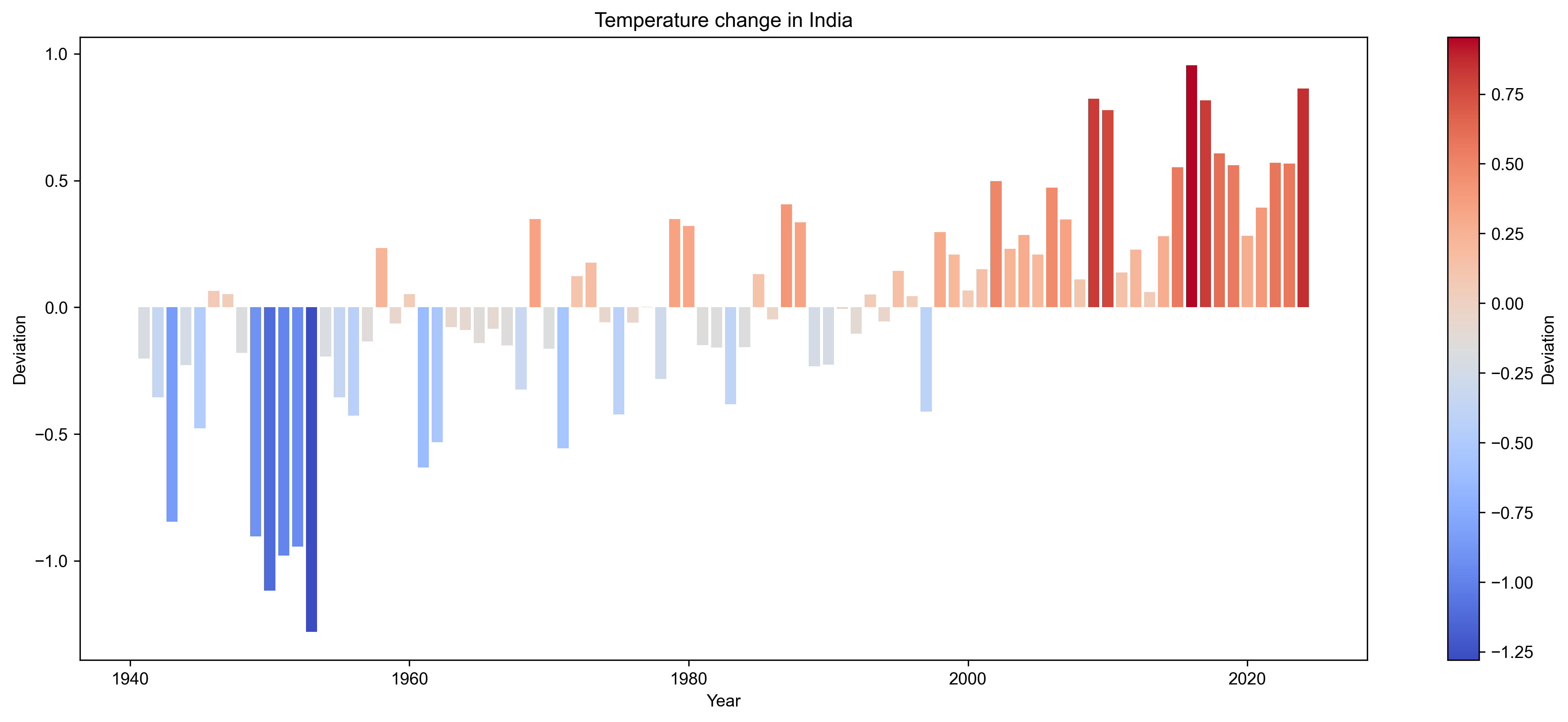
This plot shows the yearly deviation in average temperature across India from the long-term mean (1941–2024).
Bars above zero indicate warmer-than-average years, while bars below zero indicate cooler-than-average years.
The color gradient reinforces this — with warm tones for hotter years and cool tones for colder years.
Conclusion#
This example demonstrates how varunayan can be used to easily access and visualize historical climate data for a specific region — in this case, India’s average temperature from 1941 to 2024.
The visualization clearly illustrates how India’s average annual temperature has changed over the last 80+ years.
There is a noticeable upward shift in temperature deviations over time, with recent decades showing more frequent and intense warmer-than-average years.
The use of color gradients helps visually track how the climate signal has intensified over time.
By combining climate data extracted using varunayan with simple processing and visualization, we gain a compelling and accessible picture of India’s changing climate — one that is both data-driven and intuitive.