Total Precipitation and Umbrella Search Trends in India (2004–2024)

Total Precipitation and Umbrella Search Trends in India (2004–2024)#

In this notebook, we explore the relationship between rainfall patterns and public interest in umbrellas across India from 2004 to 2024.

We use varunayan to extract monthly total precipitation data from the ERA5 climate reanalysis dataset for India.

We aim to:

Compare precipitation data with Google Trends search queries for “umbrella.”
Visualize time series of both precipitation and search interest and identify potential lead-lag relationships.
Explore regional patterns in precipitation using raw high-resolution climate data (latitude-longitude based), which was obtained with the processed data from varunayan.

This study can help identify when and where umbrella demand may rise, helpful for regional sales planning.

Step 1: Extract ERA5 Total Precipitation for India#

We use the varunayan library to download monthly total precipitation (tp) for India from 2004 to 2024 at 0.1° resolution. Unit of precipitation is meters

import varunayan

varunayan.describe_variables(["total_precipitation"], dataset_type="single")

=== Variable Descriptions (SINGLE LEVELS) ===

total_precipitation:
  Category: precipitation_variables
  Description: Cumulative precipitation (convective + large-scale). Unit: meters (m) of water equivalent.

df = varunayan.era5ify_geojson(
    request_id="prec_india_2004_2024",
    variables=["total_precipitation"],
    start_date="2004-1-1",
    end_date="2024-12-31",
    json_file="https://gist.githubusercontent.com/JaggeryArray/26b6e4c09ce033305080253002c0ba76/raw/35d1ca0ca8ee64c4b5a0a8c4f22764cf6ac38bd4/india.geojson",
    frequency="monthly",
    resolution=0.1
)

============================================================
STARTING ERA5 SINGLE LEVEL PROCESSING
============================================================
Request ID: prec_india_2004_2024
Variables: ['total_precipitation']
Date Range: 2004-01-01 to 2024-12-31
Frequency: monthly
Resolution: 0.1°
GeoJSON File: C:\Users\ATHARV~1\AppData\Local\Temp\prec_india_2004_2024_temp_geojson.json


--- GeoJSON Mini Map ---

MINI MAP (68.18°W to 97.38°E, 8.13°S to 37.08°N):
┌────────────────────────────────────────┐
│········································│
│········■■■■■■■■■·······················│
│········■■■■■■■·························│
│··········■■■■··························│
│········■■■■■■■■■·······················│
│·······■■■■■■■■■■··················■■■··│
│···■■■■■■■■■■■■■■■■■■······■····■■■■■■■·│
│···■■■■■■■■■■■■■■■■■■■■■■■■··■■■■■■■····│
│·■■■■■■■■■■■■■■■■■■■■■■■■■■■····■■■·····│
│···■■■■■■■■■■■■■■■■■■■■■■■■■·····■······│
│···■■··■■■■■■■■■■■■■■■■■■■··············│
│·······■■■■■■■■■■■■■■■■·················│
│·······■■■■■■■■■■■■■■···················│
│·······■■■■■■■■■■■······················│
│·········■■■■■■■■·······················│
│·········■■■■■■■■·······················│
│··········■■■■■■························│
│···········■■■■·························│
│········································│
└────────────────────────────────────────┘
 ■ = Inside the shape
 · = Outside the shape



b27c97db6041ad9d77270d28acde6c50.zip:   0%|          | 0.00/13.8M [00:00<?, ?B/s]



eea070b0d20e28b696fd0f3f0e6d8010.zip:   0%|          | 0.00/14.0M [00:00<?, ?B/s]



2e17719d9bcf9cf9d656ef1006139c7.zip:   0%|          | 0.00/7.86M [00:00<?, ?B/s]



Saving files to output directory: prec_india_2004_2024_output
  Saved final data to: prec_india_2004_2024_output\prec_india_2004_2024_monthly_data.csv
  Saved unique coordinates to: prec_india_2004_2024_output\prec_india_2004_2024_unique_latlongs.csv
  Saved raw data to: prec_india_2004_2024_output\prec_india_2004_2024_raw_data.csv

============================================================
PROCESSING COMPLETE
============================================================

RESULTS SUMMARY:
----------------------------------------
Variables processed: 1
Time period:         2004-01-01 to 2024-12-31
Final output shape:  (252, 3)
Total complete processing time: 208.82 seconds

First 5 rows of aggregated data:
         tp  year  month
0  0.030352  2004      1
1  0.012859  2004      2
2  0.025492  2004      3
3  0.063405  2004      4
4  0.081855  2004      5

============================================================
ERA5 SINGLE LEVEL PROCESSING COMPLETED SUCCESSFULLY
============================================================

Step 2: Create Datetime Column & Convert Precipitation Units#

We create a date column from year and month and convert ERA5 tp values to millimeters by multiplying by 1000.

import pandas as pd

df['date'] = pd.to_datetime(df[['year', 'month']].assign(day=1))
df['tp'] = df['tp']*1000

Step 3: Load and Format Google Trends Data for “Umbrella”#

The dataset contains monthly search interest for the keyword “umbrella” in India from 2004 to present. We convert the Month column to datetime format for alignment.

df_trend = pd.read_csv("https://gist.githubusercontent.com/JaggeryArray/490818f9cd19336d63f9942589a61bf0/raw/92273fc7c39c5dcc71acb27242a2dd3d6b72b4ed/multiTimeline_india_googletrends_umbrella_2004-now.csv")

df_trend['date'] = pd.to_datetime(df_trend['Month'], format='%Y-%m')

Step 4: Merge Precipitation and Google Trends Data#

We perform an inner join on the date column to create a combined dataset of total precipitation and umbrella interest.

df_merged = pd.merge(df, df_trend, on='date', how='inner')

def setup_matplotlib():
    try:
        import matplotlib.pyplot as plt
    except ImportError:
        raise ImportError(
            "Matplotlib is not installed. Install it with: pip install matplotlib"
        )

    plt.rcParams["figure.dpi"] = 300
    plt.rcParams["savefig.dpi"] = 300
    plt.rcParams["font.family"] = "sans-serif"
    plt.rcParams["font.sans-serif"] = ["Arial"]
    plt.rcParams["axes.labelweight"] = "normal"

    plt.rcParams["mathtext.fontset"] = "custom"
    plt.rcParams["mathtext.rm"] = "Arial"
    plt.rcParams["mathtext.it"] = "Arial:italic"
    plt.rcParams["mathtext.bf"] = "Arial:bold"

Step 6: Visualize Total Precipitation vs Umbrella Interest#

We plot:

Total precipitation (left Y-axis)
Log-transformed umbrella search interest (right Y-axis)

This visual helps assess whether increase in precipitation is accompanied by higher umbrella search activity.

import numpy as np
import matplotlib.pyplot as plt

setup_matplotlib()

fig, ax1 = plt.subplots(figsize=(12, 5))

# Plot tp on left y-axis
ax1.plot(df_merged['date'], df_merged['tp'], color='tab:blue', marker='o', label='Total Precipitation (tp)')
ax1.set_ylabel('Total Precipitation (mm)', color='tab:blue')
ax1.tick_params(axis='y', labelcolor='tab:blue')

# Apply log transform to umbrella
umbrella_log = np.log(df_merged['umbrella'] + 1)  # Add 1 to avoid log(0)

# Plot on right y-axis
ax2 = ax1.twinx()
ax2.plot(df_merged['date'], umbrella_log, color='tab:orange', marker='s', label='umbrella (log-scaled)')
ax2.set_ylabel('Log of umbrella Trend', color='tab:orange')
ax2.tick_params(axis='y', labelcolor='tab:orange')

# Title and grid
plt.title('Total Precipitation vs Google Trends for Umbrella (Log-Transformed)')
ax1.set_xlabel('Date')
ax1.grid(True)
fig.tight_layout()

plt.show()

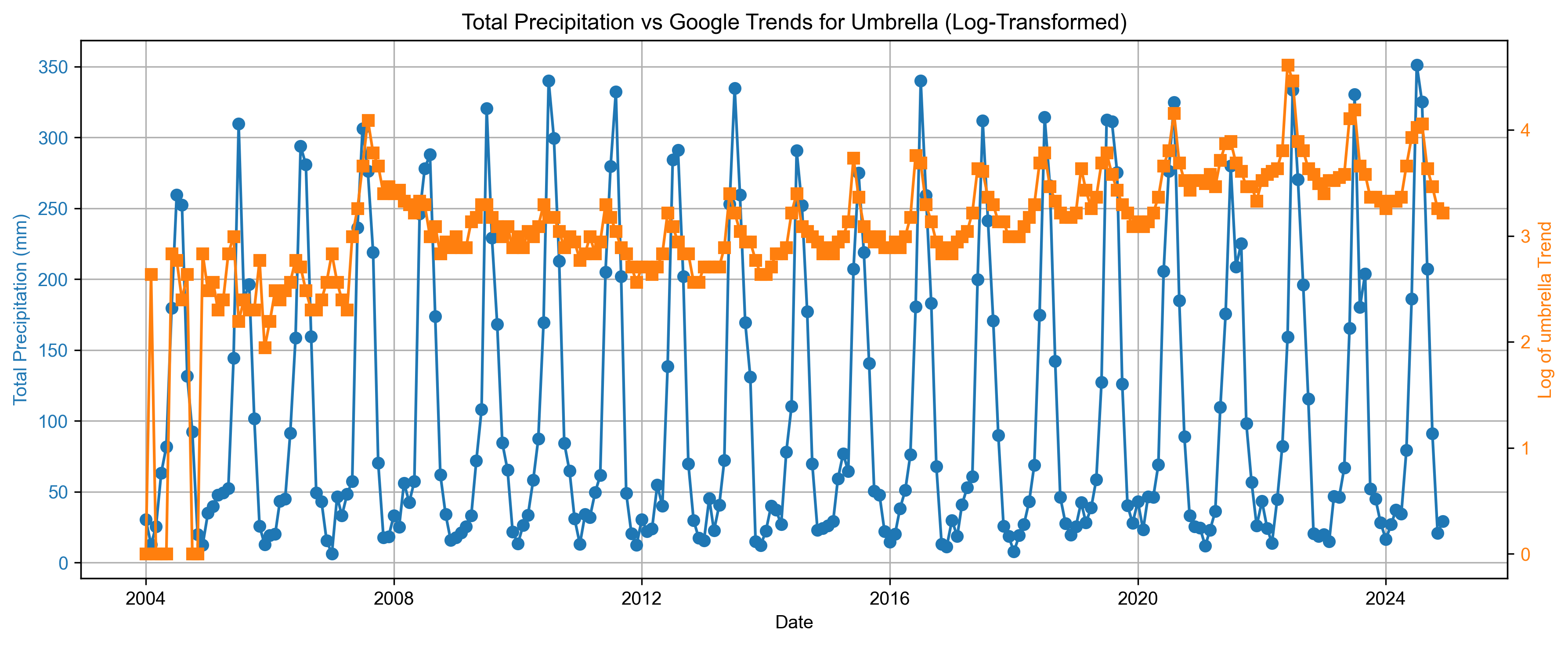
The above plot shows that there is close relation between the Google trend for the search “umbrella” and precipitation in India.

Step 7: Cross-Correlation Function (CCF)#

We normalize both tp and umbrella series and compute the cross-correlation function (CCF) across ±12 months. This reveals any leading or lagging relationships between rainfall and umbrella search interest.

import numpy as np

tp = (df_merged['tp'] - df_merged['tp'].mean()) / df_merged['tp'].std()
umbrella = (df_merged['umbrella'] - df_merged['umbrella'].mean()) / df_merged['umbrella'].std()

# Full cross-correlation
corr = np.correlate(umbrella - umbrella.mean(), tp - tp.mean(), mode='full')
lags = np.arange(-len(umbrella)+1, len(umbrella))
corr = corr / (len(umbrella) * umbrella.std() * tp.std())  # Normalize

lag_limit = 12
mask = (lags >= -lag_limit) & (lags <= lag_limit)
lags_limited = lags[mask]
corr_limited = corr[mask]

# Plot
plt.figure(figsize=(10, 5))
plt.stem(lags_limited, corr_limited)
plt.xlabel('Lag (months)')
plt.ylabel('Cross-correlation')
plt.title('CCF: Umbrella vs Total Precipitation')
plt.axvline(0, color='gray', linestyle='--')
plt.grid(True)
plt.tight_layout()
plt.show()

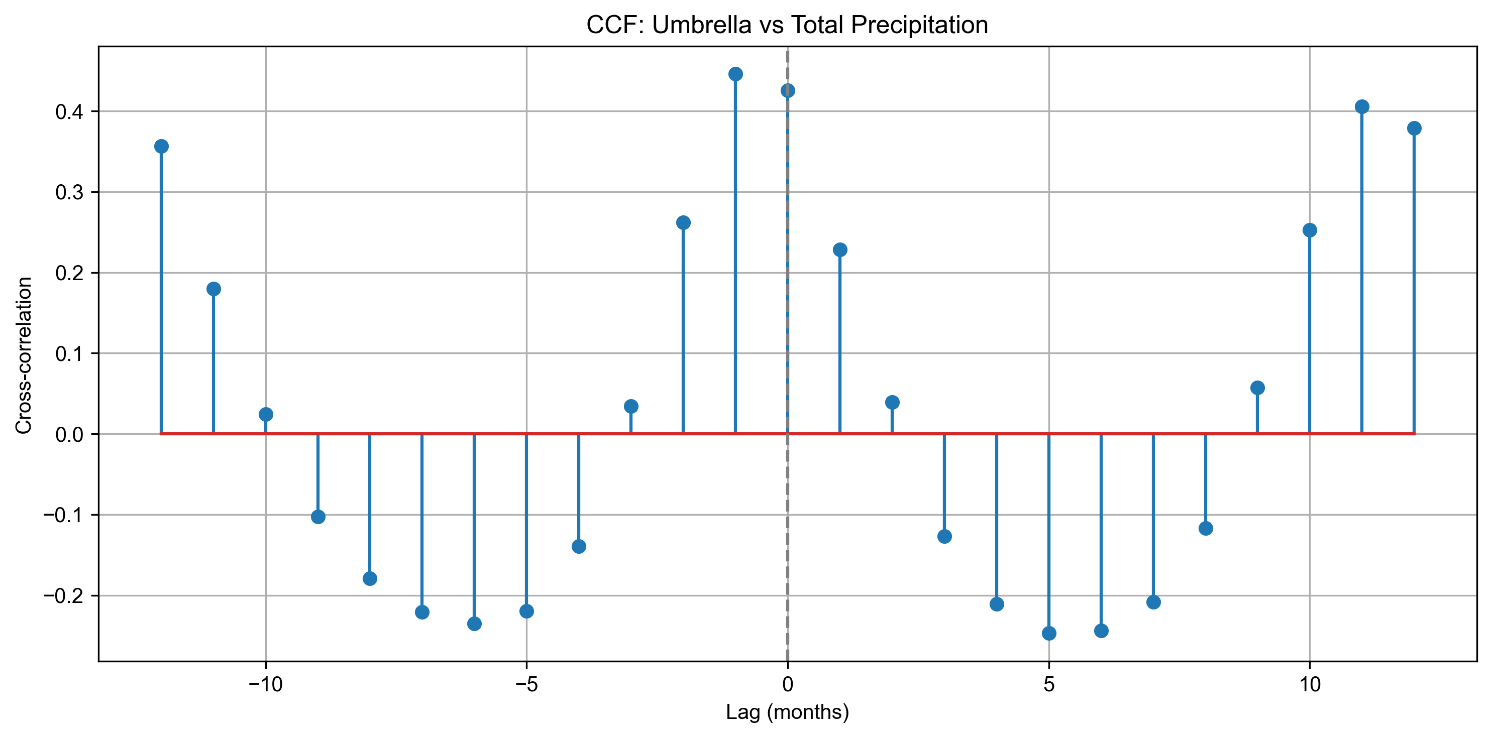
The cross-correlation plot (CCF) shows that public interest in umbrella tends to peak about one month before total precipitation reach their maximum.
This suggests that people anticipate the rain and start searching or preparing for monsoon in advance (a month before the peak to be exact).

Step 8: Load Raw ERA5 Precipitation Data#

We import raw hourly ERA5 total precipitation data (already converted to mm), and filter for June–August months to focus on India’s monsoon season.

raw_df = pd.read_csv("prec_india_2004_2024_output/prec_india_2004_2024_raw_data.csv")

Step 9: Aggregate Rainfall Across Years at Each Grid Point#

We compute the total precipitation for June, July, and August at each (latitude, longitude) grid cell averaged across all years.

raw_df['date'] = pd.to_datetime(raw_df['date'])
raw_df['tp'] = raw_df['tp'] * 1000  # Convert to mm

raw_df_rain = raw_df[raw_df['date'].dt.month.isin([6, 7, 8])]

raw_df_avg = raw_df_rain.groupby(['latitude', 'longitude'])['tp'].sum().reset_index()

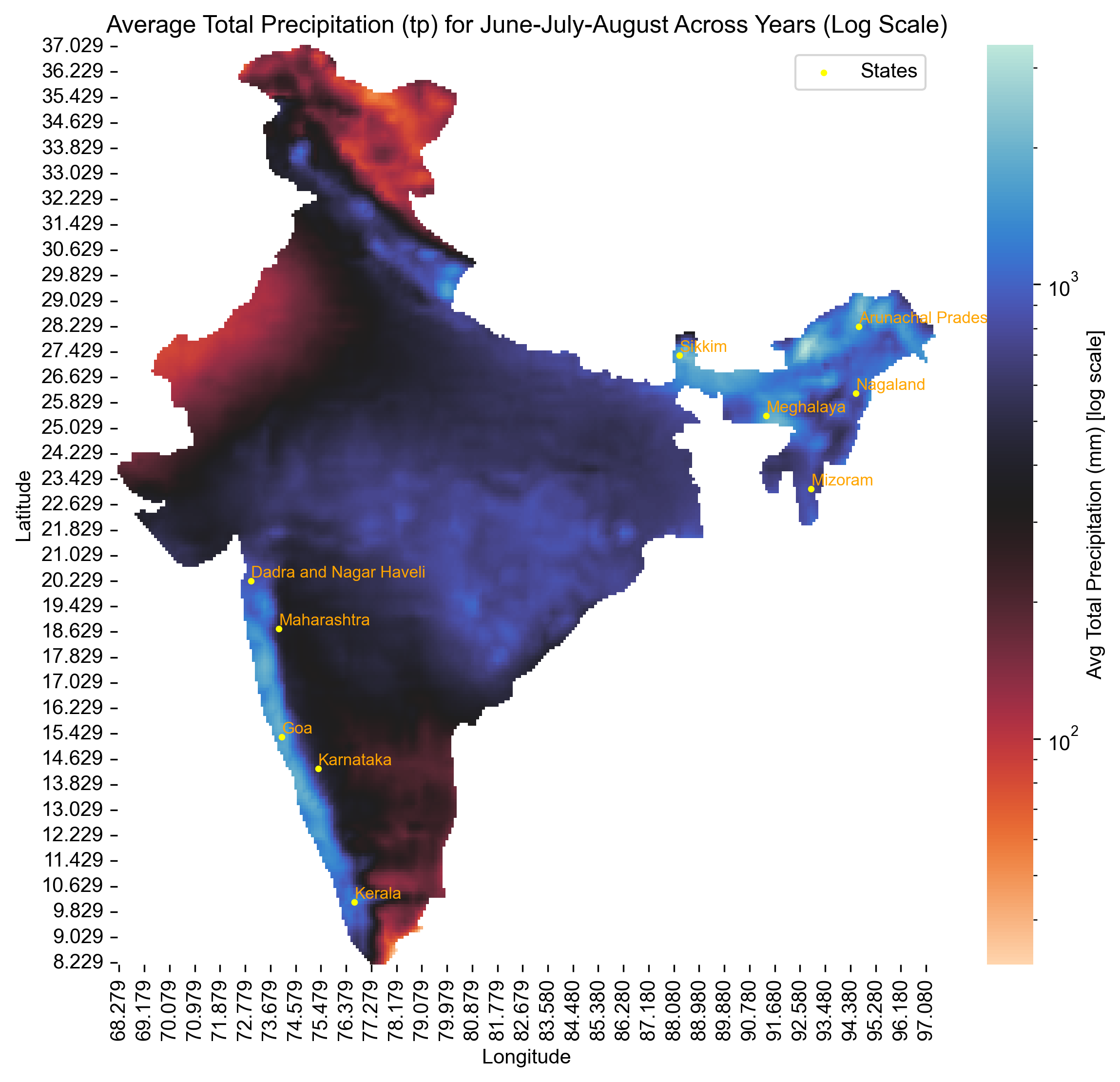
Step 10: Visualize Regional Rainfall Patterns During Monsoon#

We plot a log-scaled spatial heatmap of average June–August precipitation across India using ERA5 data from 2004 to 2024.

States with the highest interest in umbrellas during monsoon months (June–August)—based on Google Trends—are highlighted on the map.

Yellow dots mark the selected high-interest states.
Log scaling is used to simultaneously reveal both high and low precipitation zones.
This helps identify whether areas with high rainfall also show elevated umbrella-related search behavior.

import seaborn as sns
import matplotlib.pyplot as plt
import matplotlib.colors as mcolors  # For LogNorm

states = [
    "Arunachal Pradesh", "Meghalaya", "Nagaland", "Kerala", "Goa", "Sikkim", "Mizoram", "Maharashtra", "Karnataka", "Dadra and Nagar Haveli"
]

pin_lat = [
    28.2180, 25.4670, 26.1584, 10.1632, 15.2993, 27.3516, 23.1645, 18.7515, 14.3173, 20.27
]

pin_lon = [
    94.7278, 91.3662, 94.5624, 76.6413, 74.1240, 88.3239, 92.9376, 74.0139, 75.3739, 73.02
]

# Pivot data
heatmap_data = raw_df_avg.pivot(index='latitude', columns='longitude', values='tp')

# Plot heatmap with log scale
plt.figure(figsize=(8, 7.5))
ax = sns.heatmap(
    heatmap_data,
    cmap='icefire_r',
    norm=mcolors.LogNorm(vmin=heatmap_data[heatmap_data > 0].min().min(), vmax=heatmap_data.max().max()),
    cbar_kws={'label': 'Avg Total Precipitation (mm) [log scale]'}
)

# Format tick labels to 3 decimal places
ax.set_xticklabels([f"{float(label.get_text()):.3f}" for label in ax.get_xticklabels()])
ax.set_yticklabels([f"{float(label.get_text()):.3f}" for label in ax.get_yticklabels()])

plt.title('Average Total Precipitation (tp) for June-July-August Across Years (Log Scale)')
plt.xlabel('Longitude')
plt.ylabel('Latitude')
plt.gca().invert_yaxis()

lat_vals = heatmap_data.index.values
lon_vals = heatmap_data.columns.values

# Map city lat/lon to heatmap indices
pin_y = [np.argmin(np.abs(lat_vals - lat)) + 0.5 for lat in pin_lat]
pin_x = [np.argmin(np.abs(lon_vals - lon)) + 0.5 for lon in pin_lon]

plt.scatter(pin_x, pin_y, s=5, c='yellow', label='States')

# Add city names as labels
for x, y, city in zip(pin_x, pin_y, states):
    plt.text(x, y, city, fontsize=8, ha='left', va='bottom', color='orange')

plt.legend()

plt.tight_layout()
plt.show()