Comparison of ERA5 and IMD Monthly Rainfall Across Indian States (2000–2024)

In this notebook, we analyze and compare monthly precipitation patterns across Indian states using two key datasets:

• ERA5 (climate reanalysis from ECMWF)

• IMD (Indian Meteorological Department gridded rainfall data)

We focus on:

• Harmonizing ERA5 and IMD rainfall data at the state level

• Evaluating the correlation between ERA5 and IMD rainfall for each state

• Visualizing the spatial pattern of Pearson correlations to assess agreement between datasets

We use:

• varunayan for extracting ERA5 monthly precipitation (2000–2024)

• imdlib for downloading IMD monthly rainfall data

This study provides insights into how well ERA5 captures regional rainfall variability in India compared to IMD observations, which could be important for validating ERA5 use in climate research and studies for India.

Step 1: Extract ERA5 Rainfall Data for India

We use varunayan to download monthly total precipitation (tp) from the ERA5 climate reanalysis dataset for the Indian region from 2000 to 2024.

• North: 37.5°, South: 6°, East: 97.5°, West: 68°

• Resolution: 0.25°

• Frequency: Monthly

• Units: meters/day

We will be using the raw data acquired using varunayan for this analysis.

import varunayan
import pandas as pd
 
varunayan.era5ify_bbox(
    request_id='rainfall_Indian_region',
    variables=['total_precipitation'],
    start_date='2000-1-1',
    end_date='2024-12-31',
    north=37.5,
    south=6,
    east=97.5,
    west=68,
    frequency='monthly',
    resolution=0.25
)

============================================================
STARTING ERA5 SINGLE LEVEL PROCESSING
============================================================
Request ID: rainfall_Indian_region
Variables: ['total_precipitation']
Date Range: 2000-01-01 to 2024-12-31
Frequency: monthly
Resolution: 0.25°

Saving files to output directory: rainfall_Indian_region_output
  Saved final data to: rainfall_Indian_region_output\rainfall_Indian_region_monthly_data.csv
  Saved unique coordinates to: rainfall_Indian_region_output\rainfall_Indian_region_unique_latlongs.csv
  Saved raw data to: rainfall_Indian_region_output\rainfall_Indian_region_raw_data.csv

============================================================
PROCESSING COMPLETE
============================================================

RESULTS SUMMARY:
----------------------------------------
Variables processed: 1
Time period:         2000-01-01 to 2024-12-31
Final output shape:  (300, 3)
Total complete processing time: 151.79 seconds

First 5 rows of aggregated data:
         tp  year  month
0  0.036963  2000      1
1  0.033683  2000      2
2  0.044679  2000      3
3  0.055403  2000      4
4  0.128061  2000      5

============================================================
ERA5 SINGLE LEVEL PROCESSING COMPLETED SUCCESSFULLY
============================================================

	tp	year	month
0	0.036963	2000	1
1	0.033683	2000	2
2	0.044679	2000	3
3	0.055403	2000	4
4	0.128061	2000	5
...	...	...	...
295	0.261888	2024	8
296	0.177968	2024	9
297	0.133740	2024	10
298	0.088298	2024	11
299	0.068547	2024	12

300 rows × 3 columns

Step 2: Process ERA5 Monthly Rainfall Data

We process the downloaded ERA5 dataset to compute total monthly rainfall in millimeters and aggregate it at the state level.

Key steps:

1. Convert to Monthly Rainfall (mm)

   • Multiply tp (meters/day) by number of days in month × 1000

   • Final unit: millimeters per month

2. Assign State Names to Grid Points

   • Convert each (lat, lon) point to a Point geometry

   • Perform a spatial join with Indian district boundaries to assign the corresponding state

3. Statewise Monthly Aggregation

   • Compute the rainfall per state per month

The result is a dataframe (statewise_monthly_prec_era5) with:

• month, state_name, monthly_rain_mm

df_raw_prec = pd.read_csv('rainfall_Indian_region_output/rainfall_Indian_region_raw_data.csv')

import numpy as np

df_raw_prec['month'] = pd.to_datetime(df_raw_prec['date']).dt.month
df_raw_prec['date'] = pd.to_datetime(df_raw_prec['date'])
df_raw_prec['days_in_month'] = df_raw_prec['date'].dt.days_in_month

# Convert tp (precipitation in m/day) -> total monthly precipitation (in meters) -> total monthly precipitation (in mm)
df_raw_prec['tp'] = df_raw_prec['tp'] * df_raw_prec['days_in_month'] * 1000

import geopandas as gpd
from shapely.geometry import Point

df_raw_prec['geometry'] = df_raw_prec.apply(
    lambda row: Point(row['longitude'], row['latitude']), axis=1
)
gdf_prec = gpd.GeoDataFrame(df_raw_prec, geometry='geometry', crs='EPSG:4326')

url = "https://bharatviz.saketlab.in/India_LGD_Districts_simplified.geojson"
districts_gdf = gpd.read_file(url)

gdf_joined = gpd.sjoin(
    gdf_prec,
    districts_gdf[['state_name', 'geometry']],
    how='left',
    predicate='within'
)

gdf_joined = gdf_joined.dropna(subset=['state_name'])

statewise_monthly_prec_era5 = (
    gdf_joined.groupby(['date', 'state_name'], as_index=False)['tp'].mean()
    .rename(columns={'tp': 'monthly_rain_mm'})
)

statewise_monthly_prec_era5

	date	state_name	monthly_rain_mm
0	2000-01-01	A & N Islands	38.449201
1	2000-01-01	Andhra Pradesh	1.987584
2	2000-01-01	Arunachal Pradesh	147.174445
3	2000-01-01	Assam	32.347206
4	2000-01-01	Bihar	1.555414
...	...	...	...
10495	2024-12-01	Telangana	19.974696
10496	2024-12-01	Tripura	0.528455
10497	2024-12-01	Uttar Pradesh	17.636980
10498	2024-12-01	Uttarakhand	51.980734
10499	2024-12-01	West Bengal	4.839537

10500 rows × 3 columns

statewise_monthly_prec_era5.to_csv('era5_monthly_statewise_rain.csv', index=False)

Step 3: Extract IMD Gridded Rainfall Data

We use the imdlib package to download gridded IMD rainfall data over India for the same period: 2000–2024.

• Variable: 'rain'

• Format: monthwise

• Grid resolution: 0.25°

• Units: mm

This dataset provides observational rainfall data from IMD’s high-quality station network.

import imdlib as imd

start_yr = 2000
end_yr = 2024
variable = 'rain'
imd.get_data(variable, start_yr, end_yr, fn_format='monthwise')

Downloading: rain for year 2000
Downloading: rain for year 2001
Downloading: rain for year 2002
Downloading: rain for year 2003
Downloading: rain for year 2004
Downloading: rain for year 2005
Downloading: rain for year 2006
Downloading: rain for year 2007
Downloading: rain for year 2008
Downloading: rain for year 2009
Downloading: rain for year 2010
Downloading: rain for year 2011
Downloading: rain for year 2012
Downloading: rain for year 2013
Downloading: rain for year 2014
Downloading: rain for year 2015
Downloading: rain for year 2016
Downloading: rain for year 2017
Downloading: rain for year 2018
Downloading: rain for year 2019
Downloading: rain for year 2020
Downloading: rain for year 2021
Downloading: rain for year 2022
Downloading: rain for year 2023
Downloading: rain for year 2024
Download Successful !!!

<imdlib.core.IMD at 0x18e32d9a3c0>

Step 4: Process IMD Data to Statewise Monthly Rainfall

We convert the IMD gridded dataset into a statewise monthly rainfall dataset to match the format of ERA5.

Key steps:

1. Convert to DataFrame

   • Extract data from the xarray object

   • Drop missing values (-999.0)

2. Aggregate Monthly Rainfall

   • Sum rainfall for each month at each grid point

   • Create Point geometries and spatially join with state boundaries

3. Statewise Monthly Average

   • Group by state_name and month

   • Calculate average monthly rainfall

Output: statewise_monthly_prec_imd

import numpy as np

data = imd.open_data(variable, start_yr, end_yr,'monthwise')
ds = data.get_xarray()
df = ds.to_dataframe().reset_index()
df['rain'] = df['rain'].replace(-999.0, np.nan)
df

	time	lat	lon	rain
0	2000-01-01	6.5	66.50	NaN
1	2000-01-01	6.5	66.75	NaN
2	2000-01-01	6.5	67.00	NaN
3	2000-01-01	6.5	67.25	NaN
4	2000-01-01	6.5	67.50	NaN
...	...	...	...	...
159033775	2024-12-31	38.5	99.00	NaN
159033776	2024-12-31	38.5	99.25	NaN
159033777	2024-12-31	38.5	99.50	NaN
159033778	2024-12-31	38.5	99.75	NaN
159033779	2024-12-31	38.5	100.00	NaN

159033780 rows × 4 columns

df['time'] = pd.to_datetime(df['time'])
df['month'] = df['time'].dt.to_period('M')
grouped_df = df.groupby(['month', 'lat', 'lon'], as_index=False)['rain'].sum()
grouped_df

	month	lat	lon	rain
0	2000-01	6.5	66.50	0.0
1	2000-01	6.5	66.75	0.0
2	2000-01	6.5	67.00	0.0
3	2000-01	6.5	67.25	0.0
4	2000-01	6.5	67.50	0.0
...	...	...	...	...
5224495	2024-12	38.5	99.00	0.0
5224496	2024-12	38.5	99.25	0.0
5224497	2024-12	38.5	99.50	0.0
5224498	2024-12	38.5	99.75	0.0
5224499	2024-12	38.5	100.00	0.0

5224500 rows × 4 columns

import geopandas as gpd
from shapely.geometry import Point

df = grouped_df.copy()
df['geometry'] = df.apply(lambda row: Point(row['lon'], row['lat']), axis=1)
grid_gdf = gpd.GeoDataFrame(df, geometry='geometry', crs="EPSG:4326")

joined = gpd.sjoin(grid_gdf, districts_gdf[['state_name', 'geometry']], how='left', predicate='within')

statewise_monthly_prec_imd = joined.groupby(['month','state_name'], as_index=False)['rain'].mean()
statewise_monthly_prec_imd = statewise_monthly_prec_imd.dropna(subset=['state_name'])
statewise_monthly_prec_imd

	month	state_name	rain
0	2000-01	A & N Islands	0.000000
1	2000-01	Andhra Pradesh	0.055613
2	2000-01	Arunachal Pradesh	35.826280
3	2000-01	Assam	19.927342
4	2000-01	Bihar	0.523257
...	...	...	...
10495	2024-12	Telangana	17.484431
10496	2024-12	Tripura	5.540522
10497	2024-12	Uttar Pradesh	4.986236
10498	2024-12	Uttarakhand	31.285862
10499	2024-12	West Bengal	3.514762

10500 rows × 3 columns

statewise_monthly_prec_imd.to_csv('imd_monthly_statewise_rain.csv', index=False)

Step 5: Merge ERA5 and IMD Datasets

We merge the two statewise monthly rainfall datasets (ERA5 and IMD) into a common format for comparison.

• Align on: month, state_name

• Rename columns to:

  • rain_imd (from IMD)

  • rain_era5 (from ERA5)

Final merged dataset: merged_df

statewise_monthly_prec_imd['month'] = statewise_monthly_prec_imd['month'].dt.to_timestamp()

statewise_monthly_prec_era5['date'] = pd.to_datetime(statewise_monthly_prec_era5['date'])
statewise_monthly_prec_era5 = statewise_monthly_prec_era5.rename(columns={'date': 'month'})

merged_df = pd.merge(
    statewise_monthly_prec_imd,
    statewise_monthly_prec_era5,
    on=['month', 'state_name'],
    how='left'
)

merged_df = merged_df.rename(columns={
    'rain': 'rain_imd',
    'monthly_rain_mm': 'rain_era5'
})

merged_df.to_csv('merged_imd_era5_state_rain.csv', index=False)

merged_df

	month	state_name	rain_imd	rain_era5
0	2000-01-01	A & N Islands	0.000000	38.449201
1	2000-01-01	Andhra Pradesh	0.055613	1.987584
2	2000-01-01	Arunachal Pradesh	35.826280	147.174445
3	2000-01-01	Assam	19.927342	32.347206
4	2000-01-01	Bihar	0.523257	1.555414
...	...	...	...	...
10495	2024-12-01	Telangana	17.484431	19.974696
10496	2024-12-01	Tripura	5.540522	0.528455
10497	2024-12-01	Uttar Pradesh	4.986236	17.636980
10498	2024-12-01	Uttarakhand	31.285862	51.980734
10499	2024-12-01	West Bengal	3.514762	4.839537

10500 rows × 4 columns

Step 6: Compute Statewise Pearson Correlation

We compute the Pearson correlation coefficient between ERA5 and IMD rainfall for each state using the merged dataset.

• Group by state_name

• Calculate correlation between rain_imd and rain_era5

• Drop states with insufficient data (e.g., all-zero IMD values)

Final output: statewise_corr with:

• state_name, pearson_corr

statewise_corr = (
    merged_df
    .dropna(subset=['rain_imd', 'rain_era5'])
    .groupby('state_name')
    .apply(lambda df: df.loc[:, ['rain_imd', 'rain_era5']].corr().iloc[0,1])
    .reset_index(name='pearson_corr')
)

statewise_corr.to_csv('statewise_corr_imd_era5.csv', index=False)

C:\Users\Atharva Jagtap\AppData\Local\Temp\ipykernel_6688\3483317820.py:5: FutureWarning: DataFrameGroupBy.apply operated on the grouping columns. This behavior is deprecated, and in a future version of pandas the grouping columns will be excluded from the operation. Either pass `include_groups=False` to exclude the groupings or explicitly select the grouping columns after groupby to silence this warning.
  .apply(lambda df: df.loc[:, ['rain_imd', 'rain_era5']].corr().iloc[0,1])

def setup_matplotlib():
    try:
        import matplotlib.pyplot as plt
    except ImportError:
        raise ImportError(
            "Matplotlib is not installed. Install it with: pip install matplotlib"
        )

    plt.rcParams["figure.dpi"] = 300
    plt.rcParams["savefig.dpi"] = 300
    plt.rcParams["font.family"] = "sans-serif"
    plt.rcParams["font.sans-serif"] = ["Arial"]
    plt.rcParams["axes.labelweight"] = "normal"

    plt.rcParams["mathtext.fontset"] = "custom"
    plt.rcParams["mathtext.rm"] = "Arial"
    plt.rcParams["mathtext.it"] = "Arial:italic"
    plt.rcParams["mathtext.bf"] = "Arial:bold"

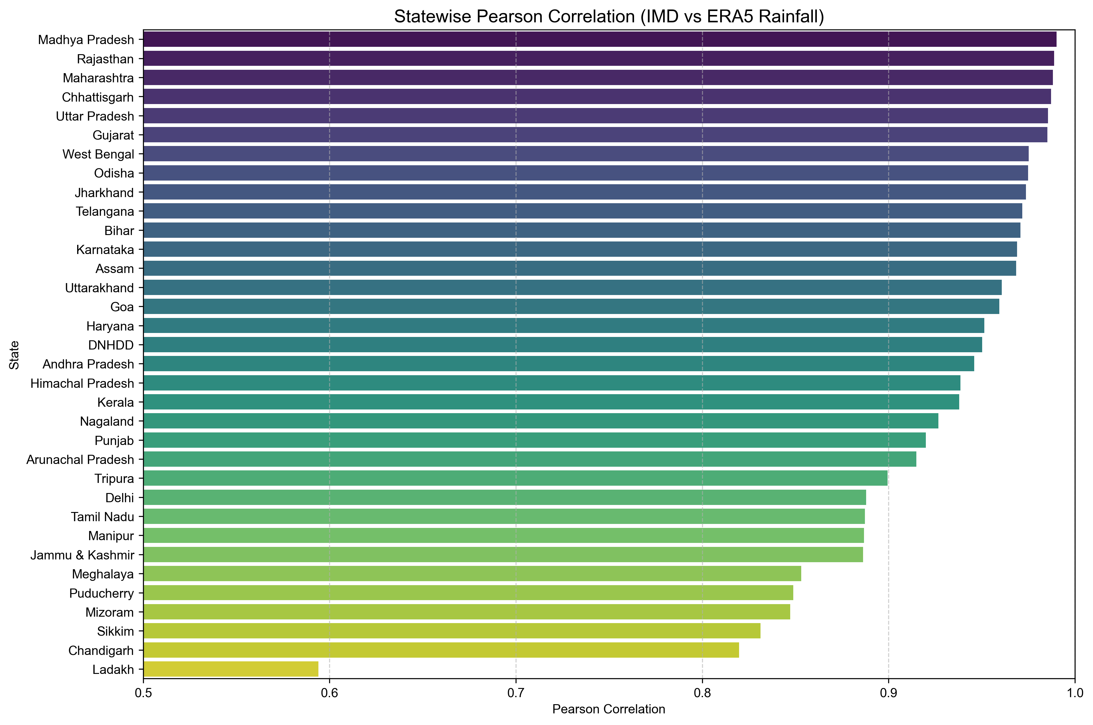
Visualize Correlation as Bar Plot

We visualize the statewise Pearson correlations using a horizontal bar chart.

• Sort states by correlation

• Highlight high agreement (closer to 1.0)

• Filter out NaN values (e.g., A & N Islands)

import pandas as pd
import matplotlib.pyplot as plt
import seaborn as sns

setup_matplotlib()

# Clean NaNs (for A & N Islands, since all the values for rainfall in IMD data are 0)
statewise_corr = statewise_corr.dropna(subset=['pearson_corr'])

statewise_corr_sorted = statewise_corr.sort_values('pearson_corr', ascending=False)

plt.figure(figsize=(12, 8))
sns.barplot(data=statewise_corr_sorted, x='pearson_corr', y='state_name', palette='viridis')

plt.title('Statewise Pearson Correlation (IMD vs ERA5 Rainfall)', fontsize=14)
plt.xlabel('Pearson Correlation')
plt.ylabel('State')
plt.xlim(0.5, 1.0)
plt.grid(axis='x', linestyle='--', alpha=0.6)
plt.tight_layout()
plt.show()

C:\Users\Atharva Jagtap\AppData\Local\Temp\ipykernel_6688\2650763813.py:13: FutureWarning:



Passing `palette` without assigning `hue` is deprecated and will be removed in v0.14.0. Assign the `y` variable to `hue` and set `legend=False` for the same effect.

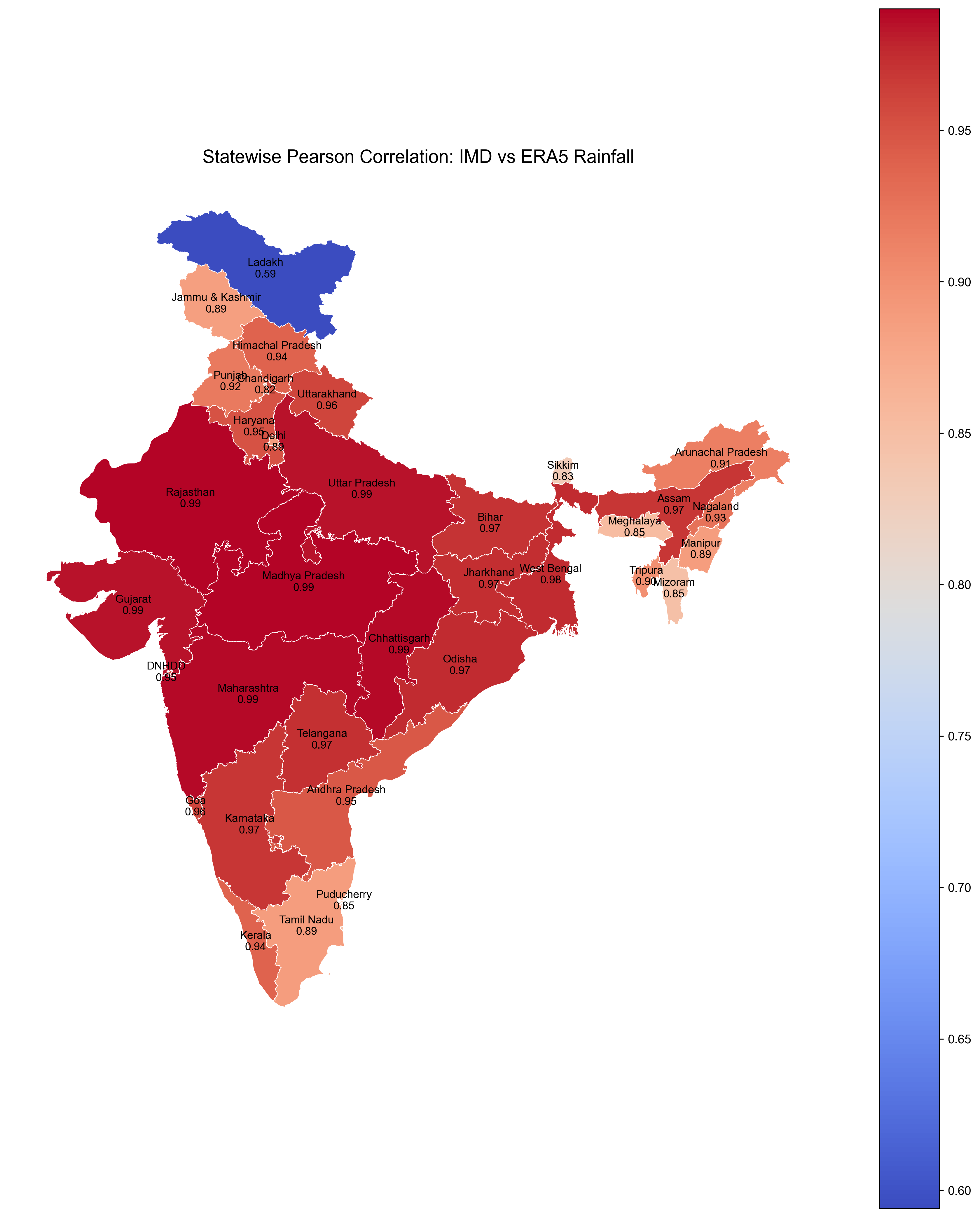
Choropleth Map of Correlation by State

We use a simplified India state GeoJSON to create a choropleth map showing the spatial pattern of correlation between ERA5 and IMD rainfall.

Features:

• Color scale (coolwarm) for correlation values

• State labels and correlation values annotated

This visualization gives a spatial perspective on how well ERA5 agrees with IMD across different regions of India.

import geopandas as gpd
import pandas as pd
import matplotlib.pyplot as plt

setup_matplotlib()

geojson_url = "https://gist.githubusercontent.com/JaggeryArray/fa31964eedb0c2da023c9485772f911a/raw/02c0644de34fbae9dbac2ba0496a00772a2c28cd/india_map_states.geojson"
gdf = gpd.read_file(geojson_url)

gdf_merged = gdf.merge(statewise_corr, on='state_name', how='left')

fig, ax = plt.subplots(figsize=(12, 14))
gdf_merged.plot(
    column='pearson_corr',
    cmap='coolwarm',
    linewidth=0.5,
    edgecolor='white',
    legend=True,
    ax=ax
)

for idx, row in gdf_merged.dropna(subset=['pearson_corr']).iterrows():
    centroid = row.geometry.centroid
    label = f"{row['state_name']}\n{row['pearson_corr']:.2f}"
    ax.text(centroid.x, centroid.y, label, fontsize=9, ha='center', va='center')

ax.set_title("Statewise Pearson Correlation: IMD vs ERA5 Rainfall", fontsize=15)
ax.axis('off')
plt.tight_layout()
plt.show()