Peak Month of Precipitation and Annual Rainfall Trends in India (2000–2024)

Peak Month of Precipitation and Annual Rainfall Trends in India (2000–2024)#

In this notebook, we explore peak month of precipitation and average annual rainfall across the Indian Region from 2000 to 2024.

We use varunayan to extract monthly total precipitation and raw high-resolution precipitation data (latitude-longitude based) from the ERA5 climate reanalysis dataset.

We aim to:

Identify the month when rainfall peaks in each region
Visualize the peak rainfall month spatially across India
Map the average annual precipitation intensity across regions

This study can help identify the peak month of rainfall and its intensity, helpful for agriculture planners and climate enthusiasts.

Step 1: Extract ERA5 Total Precipitation for India#

We use the varunayan library to download monthly total precipitation (tp) for India from 2000 to 2024 at 0.1° resolution. Unit of precipitation is meters

import varunayan
 
varunayan.era5ify_bbox(
    request_id='rainfall_Indian_region',
    variables=['total_precipitation'],
    start_date='2000-1-1',
    end_date='2024-12-31',
    north=37.1,
    south=6.3,
    east=97.4,
    west=68.1,
    frequency='monthly',
    resolution=0.1
)

============================================================
STARTING ERA5 SINGLE LEVEL PROCESSING
============================================================
Request ID: rainfall_Indian_region
Variables: ['total_precipitation']
Date Range: 2000-01-01 to 2024-12-31
Frequency: monthly
Resolution: 0.1°



66c3fdfa3d3be513f9b637537cea8222.zip:   0%|          | 0.00/14.5M [00:00<?, ?B/s]



9bad31012ee0ced1e981a10e7dd70505.zip:   0%|          | 0.00/14.6M [00:00<?, ?B/s]



573eda0df6c6b84fa185d76238e2cbba.zip:   0%|          | 0.00/14.7M [00:00<?, ?B/s]



Saving files to output directory: rainfall_Indian_region_output
  Saved final data to: rainfall_Indian_region_output\rainfall_Indian_region_monthly_data.csv
  Saved unique coordinates to: rainfall_Indian_region_output\rainfall_Indian_region_unique_latlongs.csv
  Saved raw data to: rainfall_Indian_region_output\rainfall_Indian_region_raw_data.csv

============================================================
PROCESSING COMPLETE
============================================================

RESULTS SUMMARY:
----------------------------------------
Variables processed: 1
Time period:         2000-01-01 to 2024-12-31
Final output shape:  (300, 3)
Total complete processing time: 325.50 seconds

First 5 rows of aggregated data:
         tp  year  month
0  0.035323  2000      1
1  0.033074  2000      2
2  0.044064  2000      3
3  0.054206  2000      4
4  0.128884  2000      5

============================================================
ERA5 SINGLE LEVEL PROCESSING COMPLETED SUCCESSFULLY
============================================================

	tp	year	month
0	0.035323	2000	1
1	0.033074	2000	2
2	0.044064	2000	3
3	0.054206	2000	4
4	0.128884	2000	5
...	...	...	...
295	0.266228	2024	8
296	0.180782	2024	9
297	0.133635	2024	10
298	0.087241	2024	11
299	0.068181	2024	12

300 rows × 3 columns

Step 2: Processing Monthly Precipitation Data#

We begin by loading the raw monthly precipitation data extracted using varunayan. The dataset contains gridded precipitation values (tp) for each latitude-longitude point across India.

Steps performed:#

Monthly Aggregation
- Extract the month and number of days in each entry.
- Convert tp (which is in meters/day) to total monthly precipitation in millimeters using: tp × days_in_month × 1000
Monthly Mean Grid Calculation
- Group data by location and month, and compute the mean monthly precipitation over the years (2000–2024).
- Pivot the data into a wide format — each row is a location, and each column is a month.
Peak Rainfall Month Detection
- For each location, identify the month with the highest average rainfall.
Peak Month Precipitation & Total Annual Rainfall
- Extract precipitation for the peak month at each location.
- Calculate the sum of monthly precipitation values to estimate average annual rainfall.

The resulting dataframe (result) contains:

latitude, longitude
peak_month: the month when rainfall peaks
peak_month_precip: precipitation during the peak month
avg_monsoon_precip: total average precipitation across all months

This data will be used for spatial visualizations in the next steps.

import pandas as pd

df_raw_prec = pd.read_csv('rainfall_Indian_region_output/rainfall_Indian_region_raw_data.csv')

import numpy as np

df_raw_prec['month'] = pd.to_datetime(df_raw_prec['date']).dt.month
df_raw_prec['date'] = pd.to_datetime(df_raw_prec['date'])
df_raw_prec['days_in_month'] = df_raw_prec['date'].dt.days_in_month

# Convert tp (precipitation in m/day) -> total monthly precipitation (in meters) -> total monthly precipitation (in mm)
df_raw_prec['tp'] = df_raw_prec['tp'] * df_raw_prec['days_in_month'] * 1000

monthly_mean = (
    df_raw_prec.groupby(['latitude', 'longitude', 'month'])['tp']
    .mean()
    .reset_index()
)

pivot_df = monthly_mean.pivot_table(
    index=['latitude', 'longitude'],
    columns='month',
    values='tp'
).reset_index()

pivot_df.columns.name = None

def detect_peak_month(row):
    monthly_vals = row[2:].values 
    return np.argmax(monthly_vals) + 1  

pivot_df['peak_month'] = pivot_df.apply(detect_peak_month, axis=1)

def get_peak_month_precip(row):
    return row[int(row['peak_month'])] 

pivot_df['peak_month_precip'] = pivot_df.apply(get_peak_month_precip, axis=1)

def avg_monsoon_total(row):
    peak = row['peak_month']
    monsoon_months = [1, 2, 3, 4, 5, 6, 7, 8, 9, 10, 11, 12]
    return row[monsoon_months].sum()

pivot_df['avg_monsoon_precip'] = pivot_df.apply(avg_monsoon_total, axis=1)

result = pivot_df[['latitude', 'longitude', 'peak_month', 'peak_month_precip', 'avg_monsoon_precip']]

pivot_df.to_csv('rainfall_Indian_region_output/aggregated_rainfall_coord_wise.csv', index=False)

result

	latitude	longitude	peak_month	peak_month_precip	avg_monsoon_precip
0	6.3	68.1	5	205.738712	1408.417327
1	6.3	68.2	5	206.832029	1416.722255
2	6.3	68.3	5	207.830631	1422.048801
3	6.3	68.4	5	208.726855	1424.383828
4	6.3	68.5	5	209.740787	1427.170548
...	...	...	...	...	...
90841	37.1	97.0	7	27.636770	114.003676
90842	37.1	97.1	7	29.333958	122.099992
90843	37.1	97.2	7	31.622423	132.460268
90844	37.1	97.3	7	35.038696	148.160758
90845	37.1	97.4	7	38.926897	166.562461

90846 rows × 5 columns

peak_counts = pivot_df['peak_month'].value_counts(dropna=False).sort_index()

peak_stats = pd.DataFrame({
    'month': peak_counts.index,
    'count': peak_counts.values
})

peak_stats['month'] = peak_stats['month'].apply(lambda x: int(x) if pd.notna(x) else 'NaN')

print(peak_stats)

    month  count
     2    785
     3   1091
     4    770
     5   2902
     6  12318
     7  44032
     8  14210
     9   3488
    10   1493
    11   8671
   12   1086

Step 3: Preparing State Boundaries for Mapping#

To overlay accurate state boundaries on our precipitation maps, we use a utility script to download and clean a detailed India state GeoJSON.

We fetch a script (geojson_splitter.py) from a GitHub Gist which contains a function to:
- Split and clean multi-geometry GeoJSON files.
- Ensure geometries are valid and can be plotted reliably.
The script is executed directly using exec().
We then call split_and_clean_states() on an India state boundary GeoJSON to:
- Split complex geometries (e.g., MultiPolygons).
- Save each state as a clean individual GeoJSON file for seamless overlay on maps.

These cleaned files will be used to draw precise administrative boundaries when plotting rainfall maps across India.

import requests

gist_url = "https://gist.githubusercontent.com/JaggeryArray/ab0f0ba05a65995702369fa12051ff1d/raw/3847b34e5e9105a11c1613f37dbe8330a6d4d8fa/geojson_splitter.py"

response = requests.get(gist_url)
code = response.text

exec(code)

split_and_clean_states("https://gist.githubusercontent.com/JaggeryArray/fa31964eedb0c2da023c9485772f911a/raw/02c0644de34fbae9dbac2ba0496a00772a2c28cd/india_map_states.geojson", debug_mode=False)

Downloading GeoJSON from URL...
Reading master GeoJSON...
Found 36 features across 36 unique states
Performing initial geometry cleaning...

Processing: A & N Islands
   Cleaning geometries...
   Attempting advanced repair for A & N Islands...
   Saved: split_geojsons\A_N_Islands.geojson (1 features)

Processing: Andhra Pradesh
   Cleaning geometries...
   Saved: split_geojsons\Andhra_Pradesh.geojson (1 features)

Processing: Arunachal Pradesh
   Cleaning geometries...
   Saved: split_geojsons\Arunachal_Pradesh.geojson (1 features)

Processing: Assam
   Cleaning geometries...
   Saved: split_geojsons\Assam.geojson (1 features)

Processing: Bihar
   Cleaning geometries...
   Saved: split_geojsons\Bihar.geojson (1 features)

Processing: Chandigarh
   Cleaning geometries...
   Saved: split_geojsons\Chandigarh.geojson (1 features)

Processing: Chhattisgarh
   Cleaning geometries...
   Saved: split_geojsons\Chhattisgarh.geojson (1 features)

Processing: DNHDD
   Cleaning geometries...
   Saved: split_geojsons\DNHDD.geojson (1 features)

Processing: Delhi
   Cleaning geometries...
   Saved: split_geojsons\Delhi.geojson (1 features)

Processing: Goa
   Cleaning geometries...
   Saved: split_geojsons\Goa.geojson (1 features)

Processing: Gujarat
   Cleaning geometries...
   Saved: split_geojsons\Gujarat.geojson (1 features)

Processing: Haryana
   Cleaning geometries...
   Saved: split_geojsons\Haryana.geojson (1 features)

Processing: Himachal Pradesh
   Cleaning geometries...
   Saved: split_geojsons\Himachal_Pradesh.geojson (1 features)

Processing: Jammu & Kashmir
   Cleaning geometries...
   Saved: split_geojsons\Jammu_Kashmir.geojson (1 features)

Processing: Jharkhand
   Cleaning geometries...
   Saved: split_geojsons\Jharkhand.geojson (1 features)

Processing: Kerala
   Cleaning geometries...
   Saved: split_geojsons\Kerala.geojson (1 features)

Processing: Ladakh
   Cleaning geometries...
   Saved: split_geojsons\Ladakh.geojson (1 features)

Processing: Lakshadweep
   Cleaning geometries...
   Saved: split_geojsons\Lakshadweep.geojson (1 features)

Processing: Maharashtra
   Cleaning geometries...
   Saved: split_geojsons\Maharashtra.geojson (1 features)

Processing: Manipur
   Cleaning geometries...
   Saved: split_geojsons\Manipur.geojson (1 features)

Processing: Meghalaya
   Cleaning geometries...
   Saved: split_geojsons\Meghalaya.geojson (1 features)

Processing: Mizoram
   Cleaning geometries...
   Saved: split_geojsons\Mizoram.geojson (1 features)

Processing: Nagaland
   Cleaning geometries...
   Saved: split_geojsons\Nagaland.geojson (1 features)

Processing: Odisha
   Cleaning geometries...
   Saved: split_geojsons\Odisha.geojson (1 features)

Processing: Puducherry
   Cleaning geometries...
   Saved: split_geojsons\Puducherry.geojson (1 features)

Processing: Punjab
   Cleaning geometries...
   Saved: split_geojsons\Punjab.geojson (1 features)

Processing: Rajasthan
   Cleaning geometries...
   Saved: split_geojsons\Rajasthan.geojson (1 features)

Processing: Sikkim
   Cleaning geometries...
   Saved: split_geojsons\Sikkim.geojson (1 features)

Processing: Tamil Nadu
   Cleaning geometries...
   Saved: split_geojsons\Tamil_Nadu.geojson (1 features)

Processing: Telangana
   Cleaning geometries...
   Saved: split_geojsons\Telangana.geojson (1 features)

Processing: Tripura
   Cleaning geometries...
   Saved: split_geojsons\Tripura.geojson (1 features)

Processing: Uttarakhand
   Cleaning geometries...
   Saved: split_geojsons\Uttarakhand.geojson (1 features)

Processing: Uttar Pradesh
   Cleaning geometries...
   Saved: split_geojsons\Uttar_Pradesh.geojson (1 features)

Processing: West Bengal
   Cleaning geometries...
   Saved: split_geojsons\West_Bengal.geojson (1 features)

Processing: Karnataka
   Cleaning geometries...
   Saved: split_geojsons\Karnataka.geojson (1 features)

Processing: Madhya Pradesh
   Cleaning geometries...
   Saved: split_geojsons\Madhya_Pradesh.geojson (1 features)

============================================================
FINAL SUMMARY:
Successfully saved: 36 states
Skipped due to issues: 0 -> []
Output directory: split_geojsons

def setup_matplotlib():
    try:
        import matplotlib.pyplot as plt
    except ImportError:
        raise ImportError(
            "Matplotlib is not installed. Install it with: pip install matplotlib"
        )

    plt.rcParams["figure.dpi"] = 300
    plt.rcParams["savefig.dpi"] = 300
    plt.rcParams["font.family"] = "sans-serif"
    plt.rcParams["font.sans-serif"] = ["Arial"]
    plt.rcParams["axes.labelweight"] = "normal"

    plt.rcParams["mathtext.fontset"] = "custom"
    plt.rcParams["mathtext.rm"] = "Arial"
    plt.rcParams["mathtext.it"] = "Arial:italic"
    plt.rcParams["mathtext.bf"] = "Arial:bold"

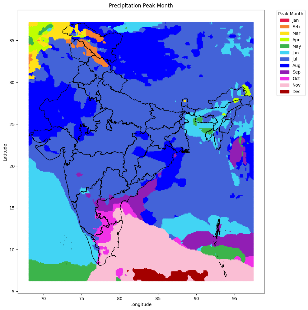
Mapping Peak Precipitation Month Across India#

We now visualize the month of peak rainfall for every coordinate in the dataset.

How it works:#

Each location’s peak precipitation month (1–12) is already computed in the earlier step.
We assign a distinct color to each month using a custom colormap.
A scatter plot of all grid points is created, with color-coded markers representing the peak rainfall month.
State boundaries (from cleaned GeoJSONs) are overlaid for better spatial reference.
A clear legend is added to map colors to month names.

This plot helps reveal the spatial variation in monsoon timing — for example, areas where the monsoon arrives early vs. those where it peaks later.

import matplotlib.pyplot as plt
import geopandas as gpd
import pandas as pd
import glob
import matplotlib.patches as mpatches
import numpy as np


month_colors = {
    0: (0.901, 0.098, 0.294),   # Jan
    1: (0.961, 0.510, 0.192),   # Feb
    2: (1.000, 0.882, 0.098),   # Mar
    3: (0.749, 1.000, 0.000),   # Apr
    4: (0.235, 0.706, 0.294),   # May
    5: (0.259, 0.831, 0.957),   # Jun
    6: (0.263, 0.388, 0.847),   # Jul
    7: (0.000, 0.000, 1.000),   # Aug
    8: (0.569, 0.118, 0.706),   # Sep
    9: (0.941, 0.196, 0.902),   # Oct
    10: (0.980, 0.745, 0.831),  # Nov
    11: (0.643, 0.000, 0.000),  # Dec
}


def get_color(row):
    base = month_colors[int(row['peak_month']) - 1]  # color for month
    return (base[0], base[1], base[2], 1)

result['plot_color'] = result.apply(get_color, axis=1)

plt.figure(figsize=(10, 12))
plt.scatter(
    result['longitude'], result['latitude'],
    c=result['plot_color'],
    s=3,
    marker='s'
)

# Overlay all state boundaries
for path in glob.glob("split_geojsons/*.geojson"):
    try:
        state_gdf = gpd.read_file(path)
        
        if state_gdf.empty:
            print(f"Skipping {path}: empty file.")
            continue
        
        # Remove invalid geometries
        state_gdf = state_gdf[state_gdf.is_valid & state_gdf.geometry.notnull()]
        
        if state_gdf.empty:
            print(f"Skipping {path}: all geometries invalid or null.")
            continue

        bounds = state_gdf.total_bounds
        if np.any(np.isnan(bounds)) or np.any(np.isinf(bounds)):
            print(f"Skipping {path}: invalid bounds.")
            continue
        
        state_gdf.boundary.plot(ax=plt.gca(), color='black', linewidth=1)
        
    except Exception as e:
        print(f"Error reading or plotting {path}: {e}")

plt.xlabel("Longitude")
plt.ylabel("Latitude")
plt.title("Precipitation Peak Month")

# Month names for legend
month_names = {
    0: 'Jan', 1: 'Feb', 2: 'Mar', 3: 'Apr',
    4: 'May', 5: 'Jun', 6: 'Jul', 7: 'Aug',
    8: 'Sep', 9: 'Oct', 10: 'Nov', 11: 'Dec'
}

# Create legend handles
legend_handles = [
    mpatches.Patch(color=month_colors[m], label=month_names[m])
    for m in range(12)
]

# Add legend box (outside plot or inside based on your preference)
plt.legend(
    handles=legend_handles,
    title="Peak Month",
    bbox_to_anchor=(1.05, 1),  # move outside right
    loc='upper left',
    borderaxespad=0.,
    frameon=True
)

plt.tight_layout()
plt.show()

C:\Users\Atharva Jagtap\AppData\Local\Temp\ipykernel_19412\945228509.py:29: SettingWithCopyWarning: 
A value is trying to be set on a copy of a slice from a DataFrame.
Try using .loc[row_indexer,col_indexer] = value instead

See the caveats in the documentation: https://pandas.pydata.org/pandas-docs/stable/user_guide/indexing.html#returning-a-view-versus-a-copy
  result['plot_color'] = result.apply(get_color, axis=1)

png

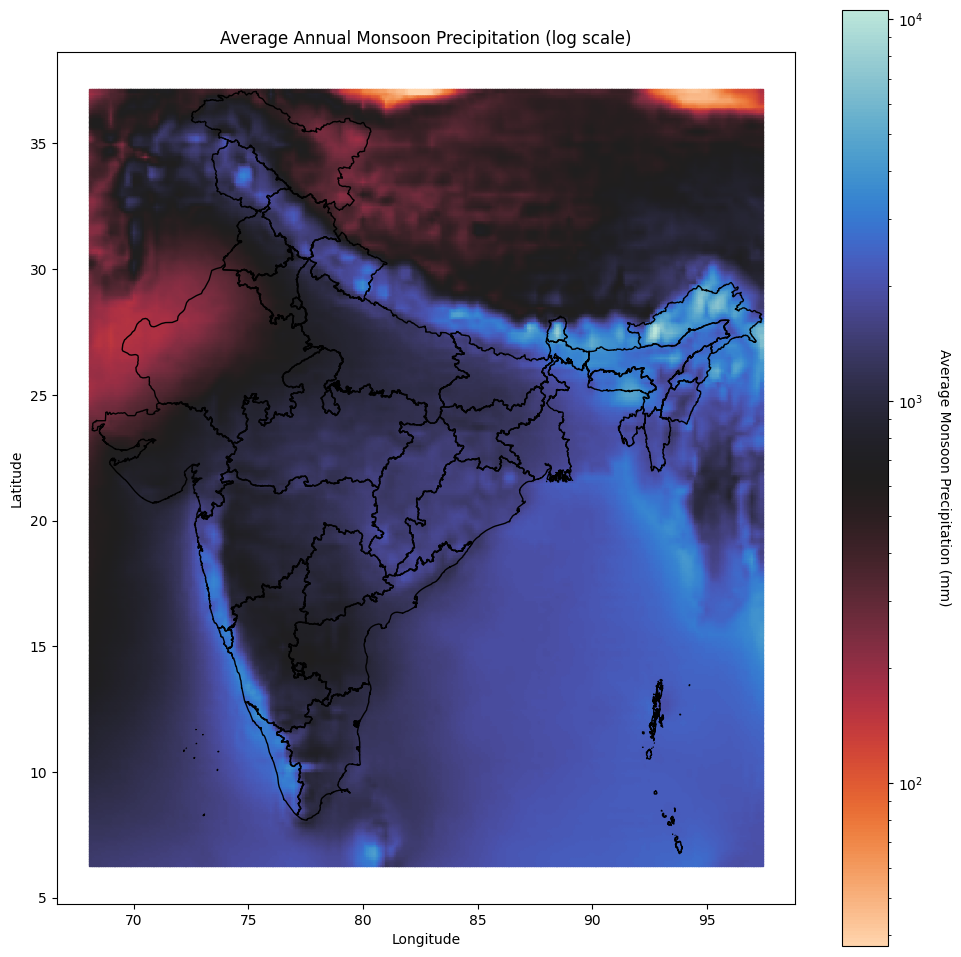
Mapping Average Annual Monsoon Precipitation#

In this step, we create a spatial heatmap of average annual monsoon precipitation across India.

How it’s done:#

Using the avg_monsoon_precip values computed earlier (in mm).
Creating a scatter plot where each point represents a grid cell and is color-coded by rainfall intensity.
The color scale is based on a logarithmic normalization, which helps in better visual contrast across regions with low vs. high rainfall.
The icefire colormap from seaborn is used for an intuitive blue-to-red transition.
We overlay state boundaries for better geographic context.

This plot helps reveal the spatial variation in annual rainfall.

import matplotlib.pyplot as plt
import geopandas as gpd
import pandas as pd
import glob
import matplotlib.patches as mpatches
import numpy as np
from matplotlib.colors import Normalize, LogNorm
import matplotlib.cm as cm
import seaborn as sns

plt.figure(figsize=(10, 12))

cmap = 'icefire_r'

min_val = result['avg_monsoon_precip'].min()
max_val = result['avg_monsoon_precip'].max()

if min_val <= 0:
    offset = 0.1
    print(f"Warning: Found values <= 0. Adding offset of {offset}")
    norm = LogNorm(vmin=max(min_val + offset, 0.1), vmax=max_val)
else:
    norm = LogNorm(vmin=min_val, vmax=max_val)

scatter = plt.scatter(
    result['longitude'], result['latitude'],
    c=result['avg_monsoon_precip'],
    cmap=cmap,
    norm=norm,
    s=3,
    marker='s'
)

# Add colorbar
cbar = plt.colorbar(scatter, shrink=0.8)
cbar.set_label('Average Monsoon Precipitation (mm)', rotation=270, labelpad=20)

# Overlay all state boundaries
for path in glob.glob("split_geojsons/*.geojson"):
    try:
        state_gdf = gpd.read_file(path)
        
        if state_gdf.empty:
            print(f"Skipping {path}: empty file.")
            continue
        
        # Remove invalid geometries
        state_gdf = state_gdf[state_gdf.is_valid & state_gdf.geometry.notnull()]
        
        if state_gdf.empty:
            print(f"Skipping {path}: all geometries invalid or null.")
            continue

        bounds = state_gdf.total_bounds
        if np.any(np.isnan(bounds)) or np.any(np.isinf(bounds)):
            print(f"Skipping {path}: invalid bounds.")
            continue
        
        state_gdf.boundary.plot(ax=plt.gca(), color='black', linewidth=1)
        
    except Exception as e:
        print(f"Error reading or plotting {path}: {e}")

# Final touches
plt.xlabel("Longitude")
plt.ylabel("Latitude")
plt.title("Average Annual Monsoon Precipitation (log scale)")

plt.tight_layout()
plt.show()

png