The problem
ERA5 and IMD give us data on regular grids (for example 0.25° × 0.25°). When we aggregate to administrative boundaries like districts, the smaller districts may contain no grid points at all, which leaves them with missing data.
districts_url <- "https://bharatviz.saketlab.org/India_LGD_districts.geojson"
districts_file <- "indian_districts.geojson"
if (!file.exists(districts_file)) {
  download.file(districts_url, districts_file, mode = "wb", timeout = 300)
}
districts_sf <- sf::st_read(districts_file, quiet = TRUE)

imd_tmax <- imd_temperature_geojson(
  request_id = "spatial_demo",
  start_year = 2023, end_year = 2023,
  geojson_file = districts_file,
  var_type = "tmax"
)

imd_spatial <- imd_tmax %>%
  group_by(longitude, latitude) %>%
  summarise(temp = mean(temperature, na.rm = TRUE), .groups = "drop")

era5_temp <- era5ify_geojson(
  request_id = "spatial_era5",
  variables = "2m_temperature",
  start_date = "2023-01-01",
  end_date = "2023-01-31",
  json_file = districts_file,
  frequency = "daily",
  resolution = 0.25
)
#>   |                                                                              |                                                                      |   0%  |                                                                              |=                                                                     |   2%  |                                                                              |===                                                                   |   4%  |                                                                              |=====                                                                 |   6%  |                                                                              |======                                                                |   9%  |                                                                              |========                                                              |  11%  |                                                                              |=========                                                             |  13%  |                                                                              |===========                                                           |  15%  |                                                                              |============                                                          |  17%  |                                                                              |==============                                                        |  20%  |                                                                              |===============                                                       |  22%  |                                                                              |=================                                                     |  24%  |                                                                              |==================                                                    |  26%  |                                                                              |====================                                                  |  28%  |                                                                              |=====================                                                 |  30%  |                                                                              |=======================                                               |  33%  |                                                                              |========================                                              |  35%  |                                                                              |==========================                                            |  37%  |                                                                              |===========================                                           |  39%  |                                                                              |=============================                                         |  41%  |                                                                              |==============================                                        |  43%  |                                                                              |================================                                      |  46%  |                                                                              |=================================                                     |  48%  |                                                                              |===================================                                   |  50%  |                                                                              |====================================                                  |  52%  |                                                                              |=========================================                             |  59%  |                                                                              |===========================================                           |  61%  |                                                                              |===============================================                       |  67%  |                                                                              |=================================================                     |  69%  |                                                                              |==================================================                    |  72%  |                                                                              |====================================================                  |  74%  |                                                                              |=====================================================                 |  76%  |                                                                              |==============================================================        |  89%  |                                                                              |================================================================      |  91%  |                                                                              |=================================================================     |  93%  |                                                                              |===================================================================   |  96%  |                                                                              |====================================================================  |  98%  |                                                                              |======================================================================| 100%

era5_spatial <- era5_temp %>%
  group_by(longitude, latitude) %>%
  summarise(temp = mean(value, na.rm = TRUE), .groups = "drop")
Visualizing grid coverage
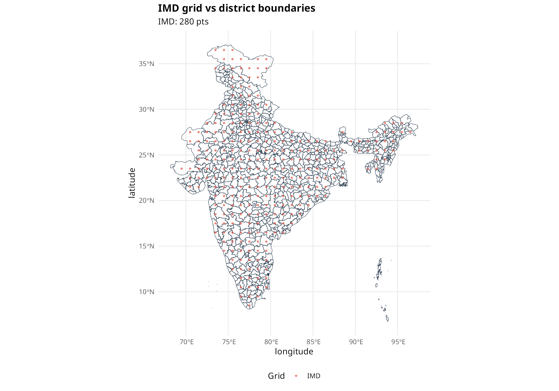
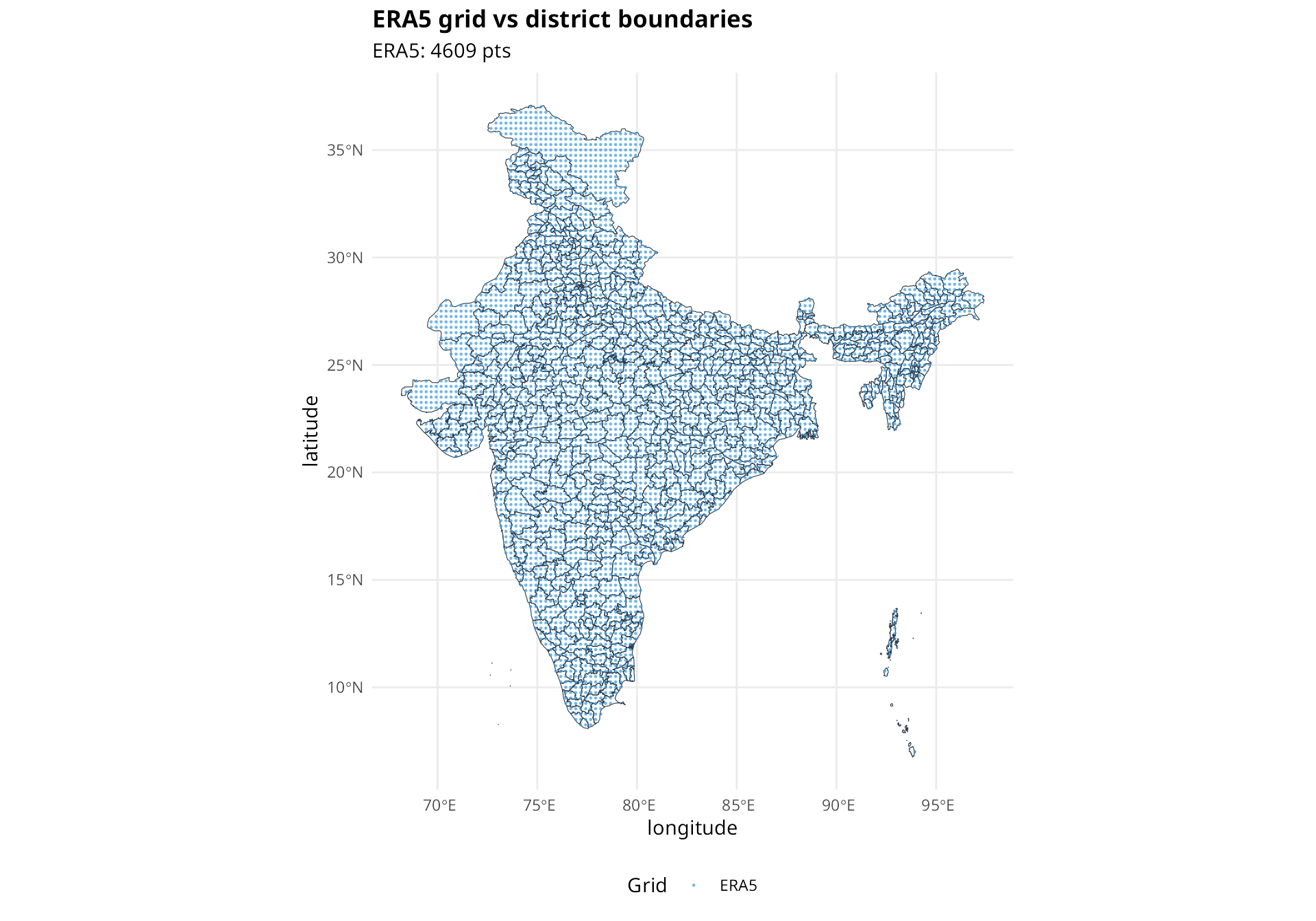
We use compare_grids() to see how the grid points align
with polygon boundaries.
compare_grids(
  IMD = imd_spatial,
  point_size = 1,
  polygons = districts_sf,
  title = "IMD grid vs district boundaries"
)
compare_grids(
  ERA5 = era5_spatial,
  colors = c(ERA5 = "#3498DB"),
  point_size = 0.5,
  polygons = districts_sf,
  title = "ERA5 grid vs district boundaries"
)
compare_grids(
  IMD = imd_spatial,
  ERA5 = era5_spatial,
  point_size = 0.5,
  polygons = districts_sf,
  title = "IMD vs ERA5 grid points"
)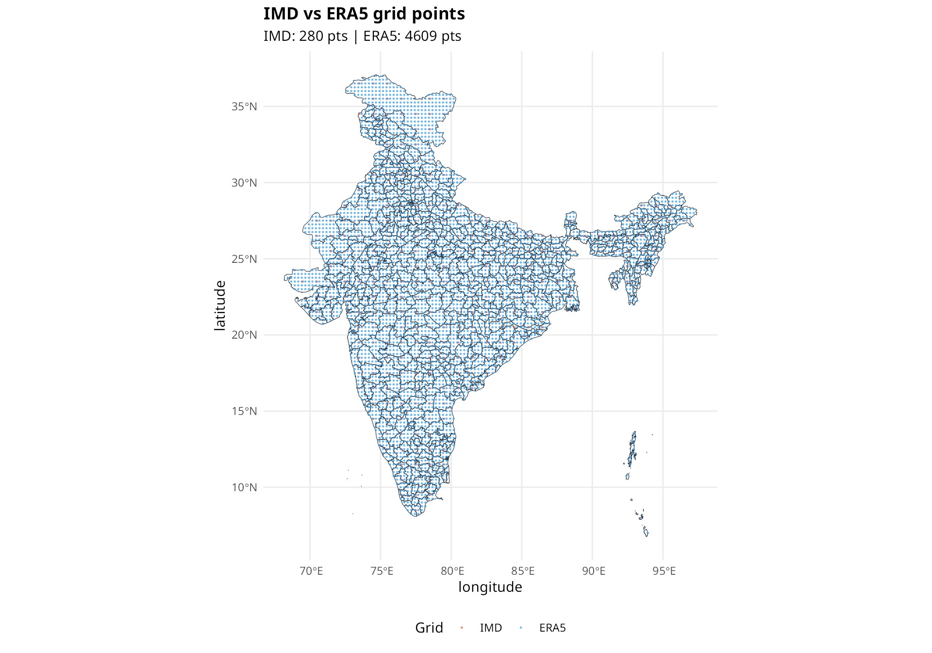
Red circles are IMD grid points, blue circles are ERA5 grid points. Many small districts have no grid points within their boundaries.
Coverage statistics
IMD coverage
imd_coverage <- check_grid_coverage(imd_spatial, districts_sf, c("state_name", "district_name"))
cat("IMD Grid Coverage:\n")
#> IMD Grid Coverage:
cat("  Total districts:", imd_coverage$total_polygons, "\n")
#>   Total districts: 785
cat("  Grid points:", imd_coverage$total_grid_points, "\n")
#>   Grid points: 280
cat("  Districts with data:", imd_coverage$polygons_with_points, "\n")
#>   Districts with data: 249
cat("  Coverage:", imd_coverage$coverage_percent, "%\n")
#>   Coverage: 31.7 %
ERA5 coverage
era5_coverage <- check_grid_coverage(era5_spatial, districts_sf, c("state_name", "district_name"))
cat("ERA5 Grid Coverage:\n")
#> ERA5 Grid Coverage:
cat("  Total districts:", era5_coverage$total_polygons, "\n")
#>   Total districts: 785
cat("  Grid points:", era5_coverage$total_grid_points, "\n")
#>   Grid points: 4635
cat("  Districts with data:", era5_coverage$polygons_with_points, "\n")
#>   Districts with data: 752
cat("  Coverage:", era5_coverage$coverage_percent, "%\n")
#>   Coverage: 95.8 %
Aggregation methods
Comparing results
make_map <- function(data, title) {
  map_sf <- districts_sf %>%
    left_join(data, by = c("state_name", "district_name"))

  ggplot(map_sf) +
    geom_sf(aes(fill = value), color = "white", linewidth = 0.05) +
    scale_fill_viridis_c(option = "plasma", na.value = "grey80", name = "°C") +
    labs(title = title) +
    theme_void() +
    theme(plot.title = element_text(hjust = 0.5, face = "bold", size = 11))
}

p1 <- make_map(result_pip, "Point-in-Polygon")
p2 <- make_map(result_nearest, "Nearest Centroid")

p1 + p2 + plot_layout(guides = "collect")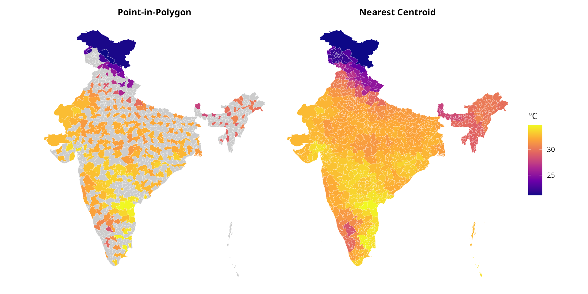
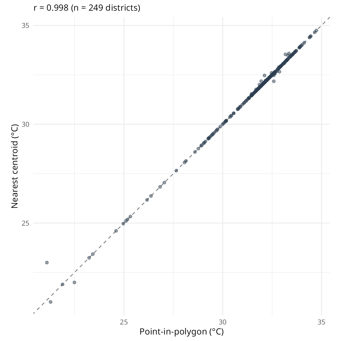
Value comparison
For districts that have data in both methods:
comparison <- result_pip %>%
  rename(pip = value) %>%
  inner_join(
    result_nearest %>% rename(nearest = value),
    by = c("state_name", "district_name")
  ) %>%
  filter(!is.na(pip) & !is.na(nearest))

cor_val <- cor(comparison$pip, comparison$nearest, use = "complete.obs")

ggplot(comparison, aes(x = pip, y = nearest)) +
  geom_abline(slope = 1, intercept = 0, linetype = "dashed", color = "grey50") +
  geom_point(alpha = 0.5, color = "#2C3E50") +
  coord_fixed() +
  labs(
    x = "Point-in-polygon (°C)",
    y = "Nearest centroid (°C)",
    subtitle = sprintf("r = %.3f (n = %d districts)", cor_val, nrow(comparison))
  ) +
  theme_minimal()