Name: varunayanR
Author: Saket Choudhary

library(varunayan)
library(dplyr)
library(ggplot2)
library(sf)
library(patchwork)

districts_url <- "https://gist.githubusercontent.com/saketkc/c2041f73fc08d39bb7b7cc39ce7b22e1/raw/2947556a7183455651d411489538452e13addb06/India_LGD_districts.geojson"
districts_file <- "indian_districts.geojson"
if (!file.exists(districts_file)) {
  download.file(districts_url, districts_file, mode = "wb", timeout = 300)
}
districts_sf <- sf::st_read(districts_file, quiet = TRUE)

Download Data

era5_temp <- era5ify_geojson(
  request_id = "era5_temp_2023",
  variables = "2m_temperature",
  start_date = "2023-01-01",
  end_date = "2023-12-31",
  json_file = districts_file,
  frequency = "daily",
  resolution = 0.25
) %>%
  mutate(date = as.Date(datetime))
#>   |                                                                              |                                                                      |   0%
#>   |                                                                              |======                                                                |   8%
#>   |                                                                              |============                                                          |  17%
#>   |                                                                              |==================                                                    |  25%
#>   |                                                                              |=======================                                               |  33%
#>   |                                                                              |=============================                                         |  42%
#>   |                                                                              |===================================                                   |  50%
#>   |                                                                              |=========================================                             |  58%
#>   |                                                                              |===============================================                       |  67%
#>   |                                                                              |====================================================                  |  75%
#>   |                                                                              |==========================================================            |  83%
#>   |                                                                              |================================================================      |  92%
#>   |                                                                              |======================================================================| 100%

imd_tmax <- imd_temperature_geojson(
  request_id = "imd_tmax_2023",
  start_year = 2023, end_year = 2023,
  geojson_file = districts_file,
  var_type = "tmax"
) %>% mutate(date = as.Date(date), var = "Tmax")

imd_tmin <- imd_temperature_geojson(
  request_id = "imd_tmin_2023",
  start_year = 2023, end_year = 2023,
  geojson_file = districts_file,
  var_type = "tmin"
) %>% mutate(date = as.Date(date), var = "Tmin")

Temperature comparison

# ERA5 daily mean temperature (spatial mean per day)
era5_daily <- era5_temp %>%
  group_by(date) %>%
  summarise(temp = mean(value, na.rm = TRUE), .groups = "drop") %>%
  mutate(source = "ERA5")

# IMD: Calculate Tmean from (Tmax + Tmin) / 2
imd_tmax_daily <- imd_tmax %>%
  group_by(date) %>%
  summarise(tmax = mean(temperature, na.rm = TRUE), .groups = "drop")

imd_tmin_daily <- imd_tmin %>%
  group_by(date) %>%
  summarise(tmin = mean(temperature, na.rm = TRUE), .groups = "drop")

imd_daily <- inner_join(imd_tmax_daily, imd_tmin_daily, by = "date") %>%
  mutate(temp = (tmax + tmin) / 2, source = "IMD") %>%
  select(date, temp, source)

temp_all <- bind_rows(era5_daily, imd_daily)

ggplot(temp_all, aes(x = date, y = temp, color = source)) +
  geom_line(alpha = 0.5) +
  geom_smooth(method = "loess", span = 0.1, se = FALSE, linewidth = 1.2) +
  scale_x_date(date_breaks = "1 month", date_labels = "%b") +
  scale_color_manual(values = c("ERA5" = "#E74C3C", "IMD" = "#2E86AB")) +
  labs(
    x = NULL, y = "Mean temperature (°C)", color = NULL,
    title = "Daily Mean temperature: ERA5 vs IMD (India, 2023)",
    subtitle = "IMD Tmean = (Tmax + Tmin) / 2"
  ) +
  theme_minimal() +
  theme(legend.position = "top")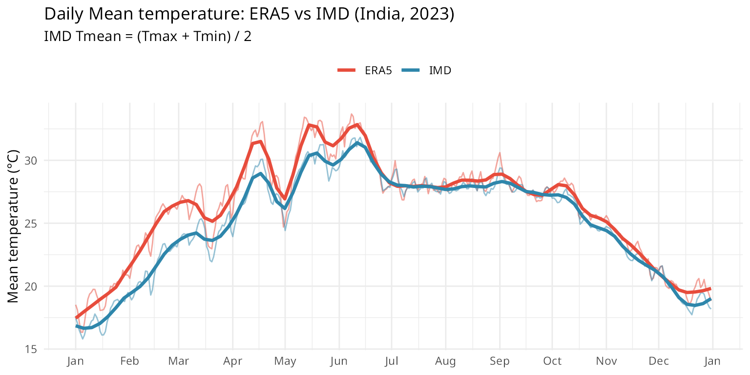

temp_wide <- inner_join(
  era5_daily %>% select(date, ERA5 = temp),
  imd_daily %>% select(date, IMD = temp),
  by = "date"
)

# Calculate correlation
cor_val <- cor(temp_wide$ERA5, temp_wide$IMD, use = "complete.obs")

ggplot(temp_wide, aes(x = IMD, y = ERA5)) +
  geom_abline(slope = 1, intercept = 0, linetype = "dashed", color = "grey40") +
  geom_point(alpha = 0.4, size = 1.5, color = "#34495E") +
  geom_smooth(method = "lm", se = TRUE, color = "#E74C3C", fill = "#E74C3C", alpha = 0.2) +
  coord_fixed() +
  labs(
    x = "IMD Mean Temperature (°C)", y = "ERA5 Mean Temperature (°C)",
    title = "ERA5 vs IMD: Daily Mean Temperature",
    subtitle = sprintf("r = %.3f", cor_val)
  ) +
  theme_minimal()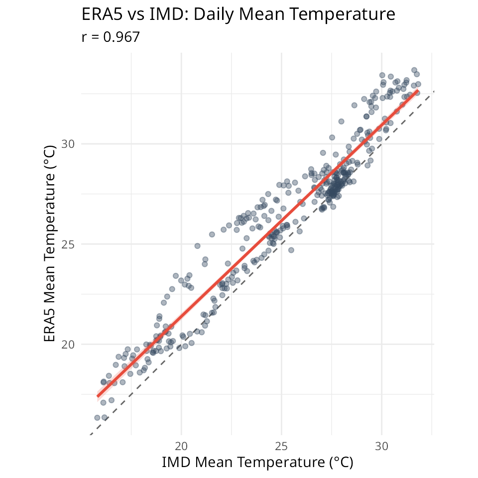

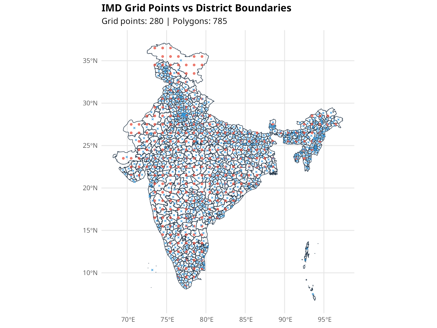
Grid Coverage Check

imd_grid <- imd_tmax %>% distinct(longitude, latitude)
coverage <- check_grid_coverage(imd_grid, districts_sf, c("state_name", "district_name"))
cat(coverage$summary, "\n")
#> 249/785 polygons (31.7%) contain at least one grid point

visualize_grid_overlap(
  imd_grid, districts_sf,
  show_centroids = TRUE,
  title = "IMD Grid Points vs District Boundaries"
)

ERA5 vs IMD

# ERA5 mean temp by district (using nearest centroid for better coverage)
era5_spatial <- era5_temp %>%
  group_by(longitude, latitude) %>%
  summarise(temp = mean(value, na.rm = TRUE), .groups = "drop")

era5_districts <- aggregate_to_polygons(
  era5_spatial, districts_sf, "temp",
  method = "nearest_centroid",
  polygon_id_cols = c("state_name", "district_name")
)

# IMD mean temp by district: (Tmax + Tmin) / 2
imd_tmax_spatial <- imd_tmax %>%
  group_by(longitude, latitude) %>%
  summarise(tmax = mean(temperature, na.rm = TRUE), .groups = "drop")

imd_tmin_spatial <- imd_tmin %>%
  group_by(longitude, latitude) %>%
  summarise(tmin = mean(temperature, na.rm = TRUE), .groups = "drop")

imd_mean_spatial <- inner_join(imd_tmax_spatial, imd_tmin_spatial, by = c("longitude", "latitude")) %>%
  mutate(temp = (tmax + tmin) / 2)

imd_districts <- aggregate_to_polygons(
  imd_mean_spatial, districts_sf, "temp",
  method = "nearest_centroid",
  polygon_id_cols = c("state_name", "district_name")
)

make_temp_map <- function(districts_sf, data, title, limits) {
  map_sf <- districts_sf %>% left_join(data, by = c("state_name", "district_name"))
  ggplot(map_sf) +
    geom_sf(aes(fill = value), color = "white", linewidth = 0.1) +
    scale_fill_gradient2(
      low = "#2166AC", mid = "#F7F7F7", high = "#B2182B",
      midpoint = mean(limits),
      limits = limits, name = "°C", na.value = "grey80"
    ) +
    labs(title = title) +
    theme_void() +
    theme(plot.title = element_text(hjust = 0.5, face = "bold", size = 11))
}

temp_limits <- range(c(era5_districts$value, imd_districts$value), na.rm = TRUE)

p1 <- make_temp_map(districts_sf, era5_districts, "ERA5", temp_limits)
p2 <- make_temp_map(districts_sf, imd_districts, "IMD", temp_limits)

p1 + p2 + plot_layout(ncol = 2, guides = "collect") &
  theme(legend.position = "right")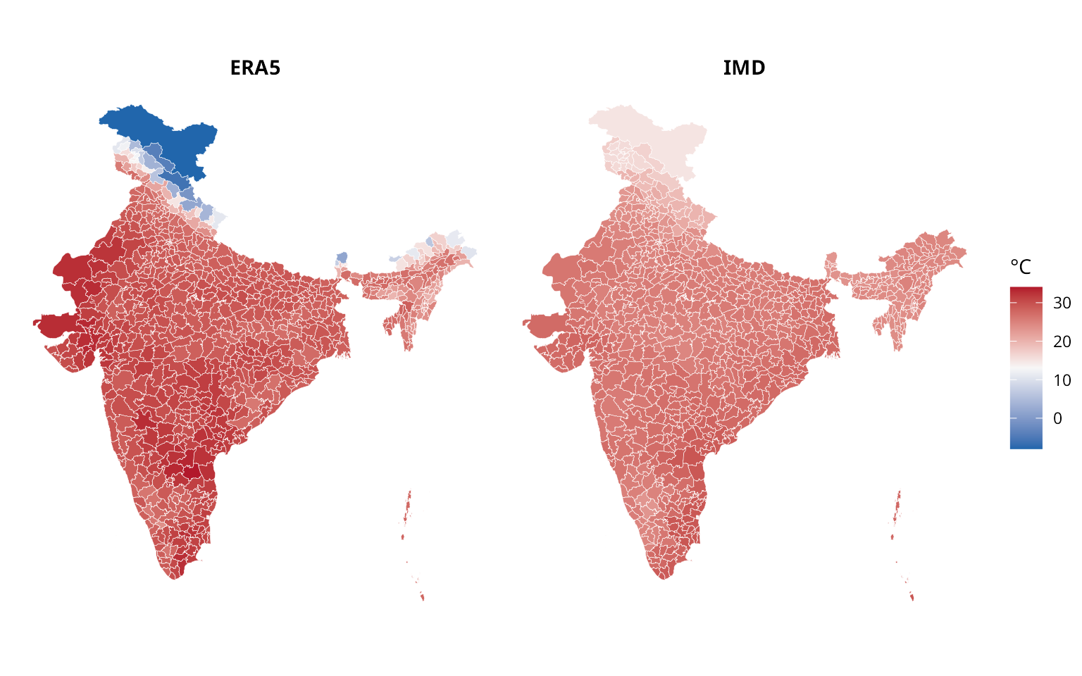

Using BharatViz

BharatViz provides publication-ready choropleth maps of India.

# Prepare district-level data for BharatViz API
era5_api_data <- era5_districts %>%
  filter(!is.na(value)) %>%
  transmute(state = state_name, district = district_name, value = round(value, 1))

imd_api_data <- imd_districts %>%
  filter(!is.na(value)) %>%
  transmute(state = state_name, district = district_name, value = round(value, 1))

# not run in knit mode
library(R6)
library(gridExtra)
source("https://raw.githubusercontent.com/saketlab/bharatviz/refs/heads/main/server/examples/bharatviz.R")

bv <- BharatViz$new()

era5_result <- bv$generate_districts_map(
  era5_api_data,
  map_type = "LGD",
  title = "ERA5 Mean Temp (2023)",
  legend_title = "°C"
)
imd_result <- bv$generate_districts_map(
  imd_api_data,
  map_type = "LGD",
  title = "IMD Mean Temp (2023)",
  legend_title = "°C"
)

era5_grob <- bv$get_grob(era5_result)
imd_grob <- bv$get_grob(imd_result)

grid.arrange(era5_grob, imd_grob, ncol = 2)

ERA5 vs IMD: Temperature comparison (2023)

Download Data

Temperature comparison

Grid Coverage Check

ERA5 vs IMD

Using BharatViz