library(anumaan)
library(dplyr)

Overview

This vignette covers the exploratory data analysis (EDA) layer. It sits between the two other pipelines: it is run on data that has already been through Preprocessing, and it is what a stewardship team typically reviews before committing to DALY burden estimation. It does not transform data (like Pipeline 1) or estimate burden (like Pipeline 3) – it only visualises what is already there, to catch data-quality problems and characterise the cohort before further modelling.

All functions in this layer are named plot_* (with the shared styling helper eda_theme()), which is deliberately distinct from the prep_* (Pipeline 1) and daly_* (Pipeline 3) naming used elsewhere in the package.

Most plot_* functions here share a common mode argument:

"faceted" – one panel per centre (the default for most functions)
"overall" – all centres pooled into a single chart
"single" – one specific centre, passed via center = "..."

and a common syndrome_col/syndrome_name pair for restricting the plot to one infectious syndrome (e.g. syndrome_name = "BSI") when that column is available.

Connecting from Pipeline 1

The plot_* functions’ default column names (organism_name, antibiotic_value, PatientInformation_id, …) are convenience defaults for raw-ish data – they do not automatically match the standardised column names Preprocessing actually produces. When passing real preprocessed output into these functions, map the arguments to Pipeline 1’s real output columns explicitly:

EDA argument	Pipeline 1’s actual output column
`patient_col`	`patient_id`
`organism_col`	`organism_normalized` (from `prep_standardize_organisms()`)
`antibiotic_col`	`antibiotic_normalized` (from `prep_standardize_antibiotics()`)
`value_col`	`ast_value_harmonized` (from `prep_harmonize_ast()`)
`sample_col`	`specimen_normalized` (from `prep_standardize_specimens()`)
`agebin_col`	`Age_bin` (from `prep_assign_age_bins()`)
`age_col`	`Age` (from `prep_fill_age()`)
`admission_col`	`date_of_admission`
`culture_col`	`date_of_culture`
`discharge_col`	`date_of_final_outcome`
`center_col`	`center_name` (a user-supplied raw column – Pipeline 1 does not invent hospital identity, it just carries it through)
`outcome_col`	`final_outcome` (the raw outcome text persists unchanged; `prep_standardize_final_outcome()` adds a separate `outcome_std` column alongside it rather than replacing it)

Every example below uses these Pipeline-1-aligned names, with the arguments passed explicitly rather than relying on defaults.

A Small Synthetic Dataset

The examples below use a small synthetic long-format dataset (one row per isolate x antibiotic) with the same column names Pipeline 1 would hand off – as if it were the output of the Preprocessing vignette’s prepped object, scaled up to two hospitals so the mode = "faceted" examples have something to facet over.

set.seed(42)
n_pts <- 60
centers <- c("General Hospital", "City Medical Center")
organisms <- c("Escherichia coli", "Klebsiella pneumoniae",
                "Staphylococcus aureus", "Pseudomonas aeruginosa")
antibiotics <- c("Amikacin", "Ciprofloxacin", "Meropenem", "Ceftriaxone")

eda_data <- data.frame(
  patient_id             = paste0("pt_", sprintf("%03d", rep(1:n_pts, each = 3))),
  center_name            = rep(sample(centers, n_pts, replace = TRUE), each = 3),
  organism_normalized    = rep(sample(organisms, n_pts, replace = TRUE), each = 3),
  antibiotic_normalized  = rep(antibiotics, length.out = n_pts * 3),
  ast_value_harmonized   = sample(c("R", "S"), n_pts * 3, replace = TRUE, prob = c(0.4, 0.6)),
  specimen_normalized    = rep(sample(c("Blood", "Urine", "Sputum"), n_pts, replace = TRUE), each = 3),
  final_outcome          = rep(sample(c("Death", "Discharged", "LAMA", "Transferred to other hospital"),
                                       n_pts, replace = TRUE, prob = c(0.15, 0.65, 0.1, 0.1)), each = 3),
  date_of_final_outcome  = rep(as.Date("2024-01-01") + sample(1:300, n_pts, replace = TRUE), each = 3),
  is_polymicrobial       = rep(sample(c(0, 1), n_pts, replace = TRUE, prob = c(0.75, 0.25)), each = 3),
  date_of_admission      = rep(as.Date("2024-01-01") + sample(1:300, n_pts, replace = TRUE), each = 3),
  location               = rep(sample(c("ICU", "Ward"), n_pts, replace = TRUE), each = 3),
  infection_type         = rep(sample(c("HAI", "CAI"), n_pts, replace = TRUE), each = 3),
  Age_bin                = rep(sample(c("<1", "1-5", "18-45", "45-65", "65+"), n_pts, replace = TRUE), each = 3),
  Age                    = rep(sample(0:85, n_pts, replace = TRUE), each = 3),
  infectious_syndrome    = rep(sample(c("BSI", "UTI", "RTI"), n_pts, replace = TRUE), each = 3),
  stringsAsFactors = FALSE
)
eda_data$date_of_culture <- eda_data$date_of_admission + sample(0:5, nrow(eda_data), replace = TRUE)

nrow(eda_data)
#> [1] 180

Theme

eda_theme() is the shared visual style behind every plot in this vignette – based on ggpubr::theme_pubr() when ggpubr is installed, falling back to ggplot2::theme_bw() otherwise. You do not normally call it directly; it is applied internally by every plot_* function.

eda_theme(base_size = 14)

Organism and Susceptibility Overview

Top organisms

plot_top_organisms(
  eda_data, n = 3, mode = "faceted",
  patient_col = "patient_id", organism_col = "organism_normalized", center_col = "center_name"
)

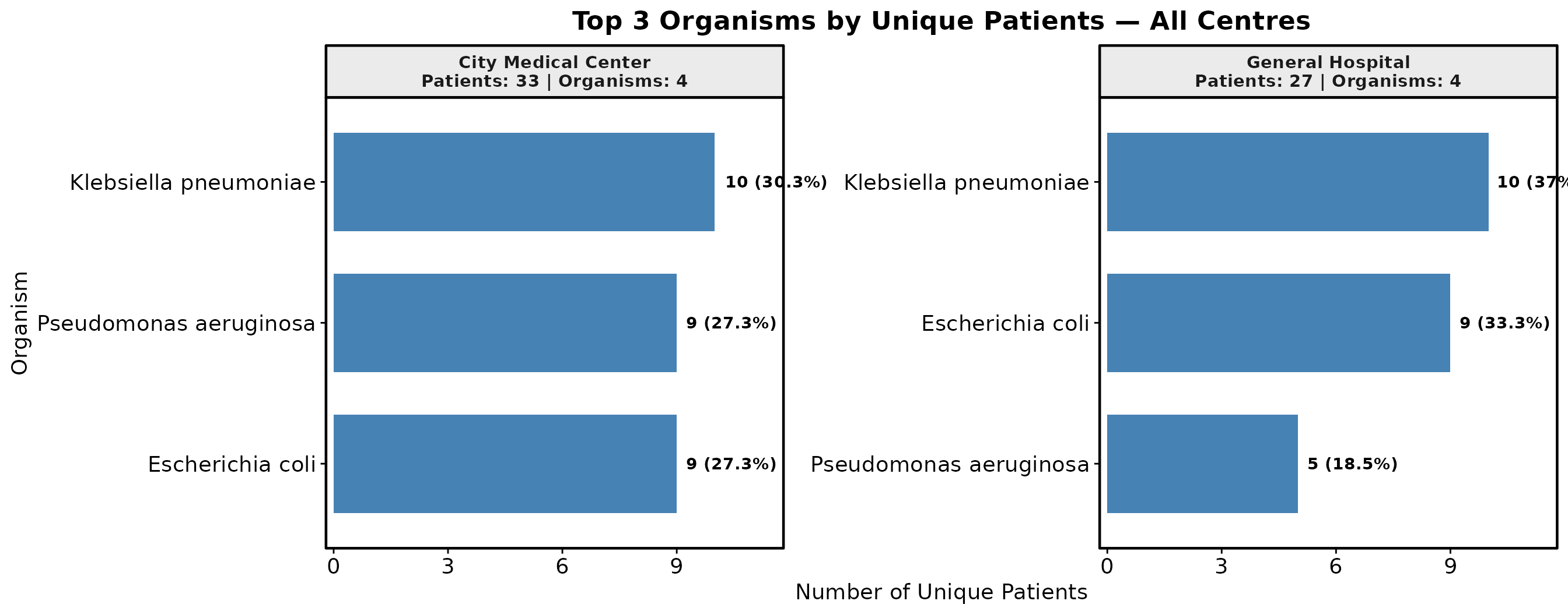
Pool across all centres with mode = "overall", or restrict to one centre with mode = "single", center = "General Hospital".

Susceptibility pattern (stacked R/S bars)

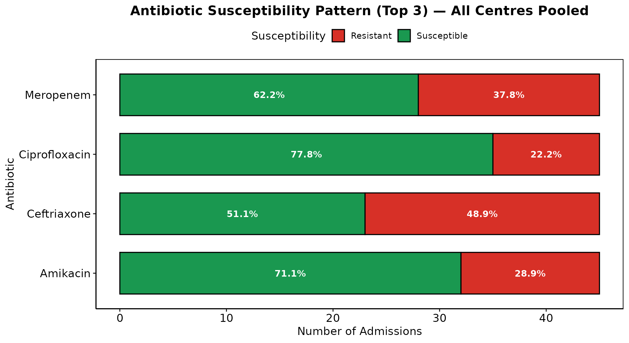
plot_abx_susceptibility() applies a worst-phenotype rule: if a patient has multiple records for the same organism-antibiotic combination, a single R result marks the whole episode as R, so repeat cultures from one infection episode are not double-counted.

plot_abx_susceptibility(
  eda_data, n = 3, mode = "overall",
  patient_col = "patient_id", antibiotic_col = "antibiotic_normalized",
  value_col = "ast_value_harmonized", organism_col = "organism_normalized",
  center_col = "center_name"
)

Resistance heatmap

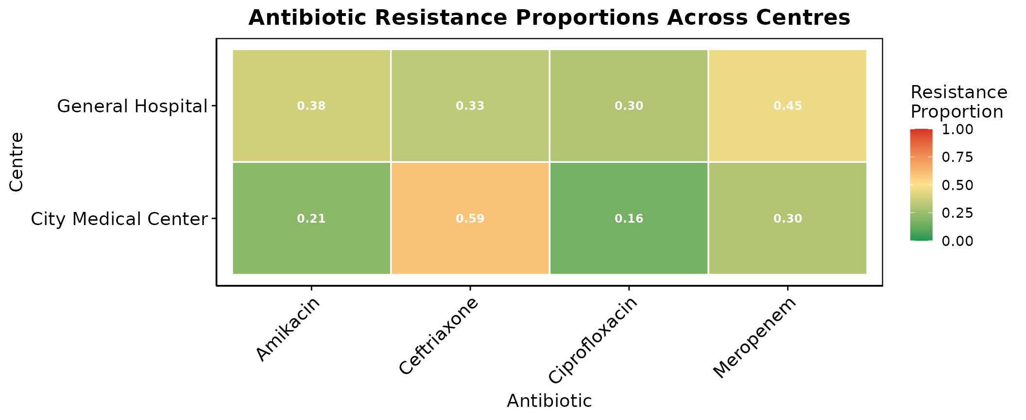
plot_abx_heatmap(
  eda_data, mode = "all",
  patient_col = "patient_id", antibiotic_col = "antibiotic_normalized",
  value_col = "ast_value_harmonized", organism_col = "organism_normalized",
  center_col = "center_name"
)

Resistance by specimen type

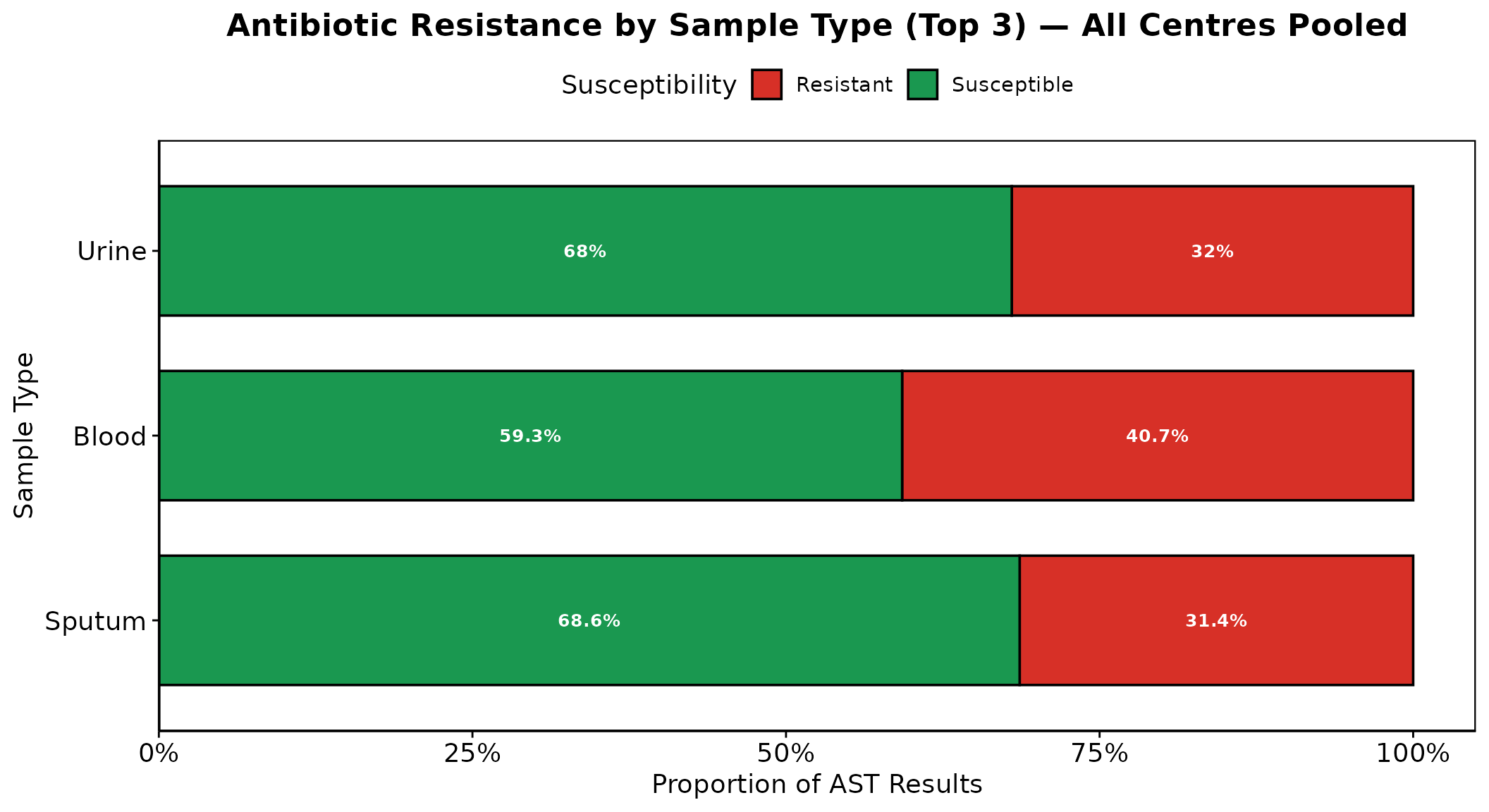
plot_resistance_by_sample(
  eda_data, n = 3, mode = "overall",
  patient_col = "patient_id", sample_col = "specimen_normalized",
  organism_col = "organism_normalized", antibiotic_col = "antibiotic_normalized",
  value_col = "ast_value_harmonized", center_col = "center_name"
)

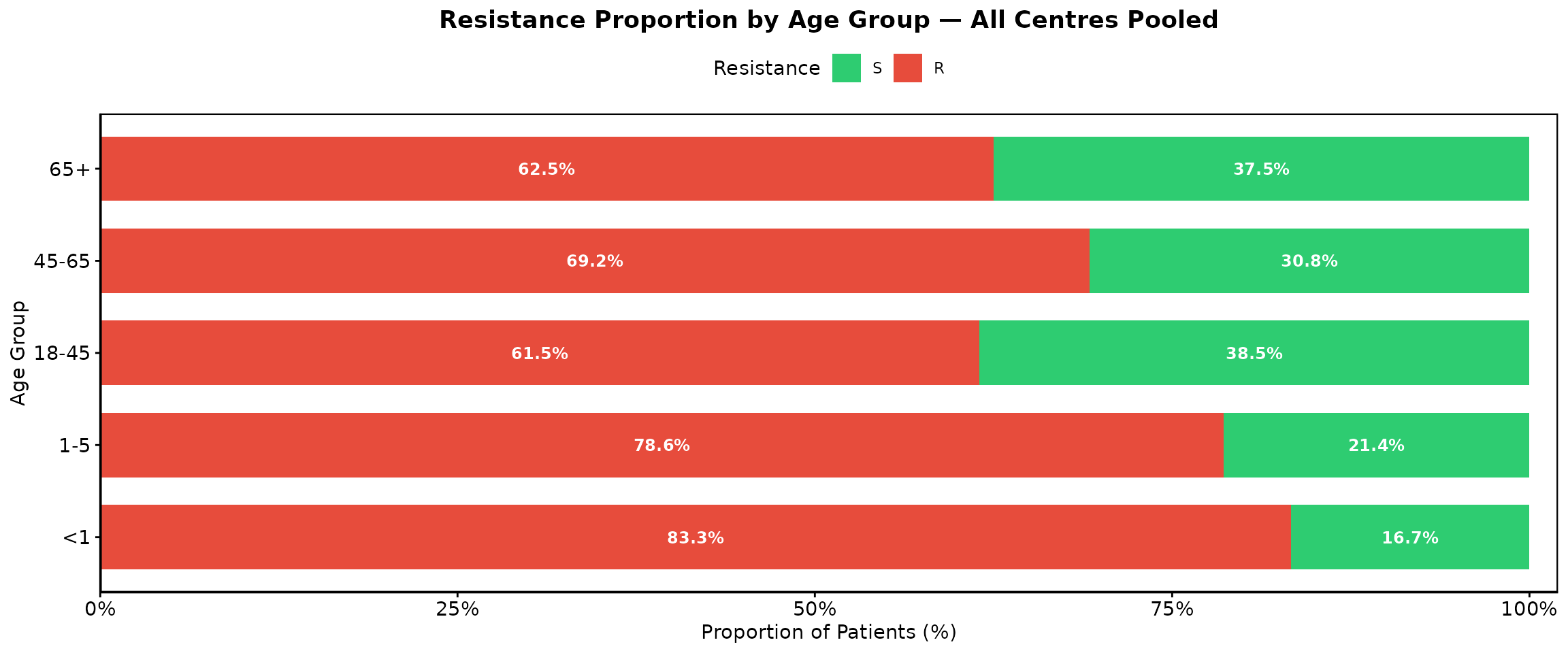
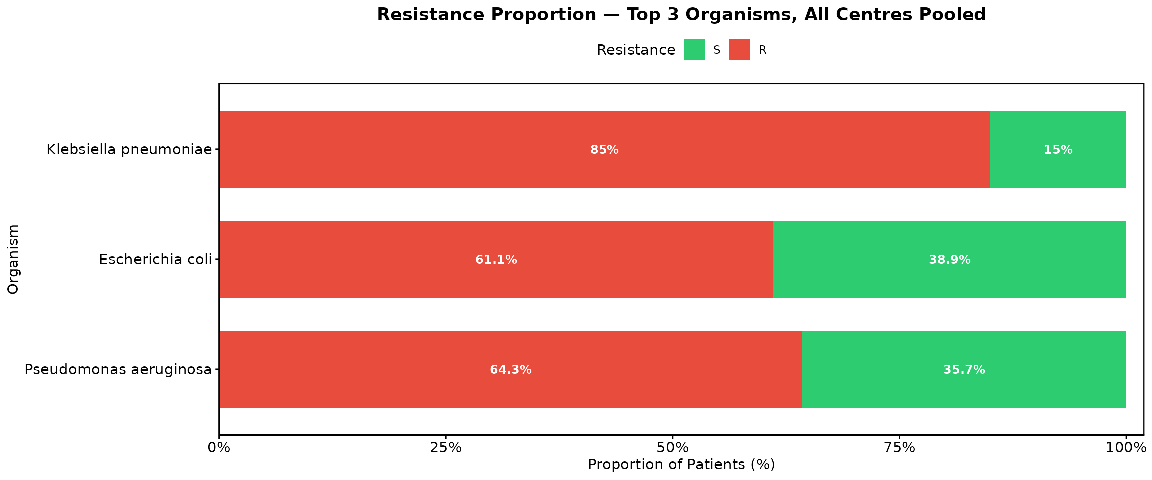
Resistance by age bin and by organism

plot_resistance_by_agebin(
  eda_data, mode = "overall",
  patient_col = "patient_id", organism_col = "organism_normalized",
  antibiotic_col = "antibiotic_normalized", value_col = "ast_value_harmonized",
  agebin_col = "Age_bin", center_col = "center_name"
)

plot_resistance_by_organism(
  eda_data, n = 3, mode = "overall",
  patient_col = "patient_id", organism_col = "organism_normalized",
  antibiotic_col = "antibiotic_normalized", value_col = "ast_value_harmonized",
  center_col = "center_name"
)

Outcomes

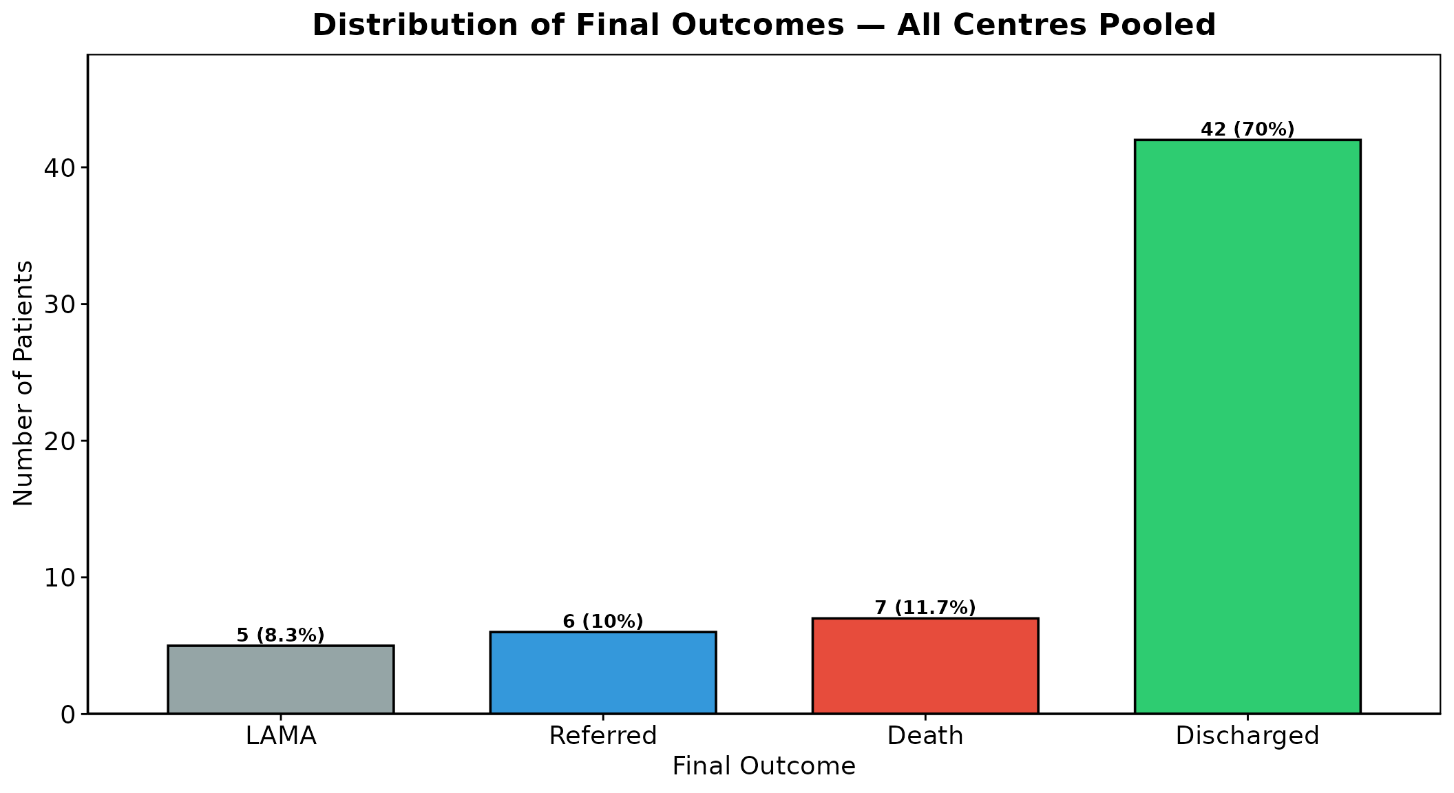
Overall distribution

By default merge_referred = TRUE recodes "Transferred to other hospital" to "Referred", since both represent the same clinical event across centres.

plot_outcome_distribution(
  eda_data, mode = "overall",
  patient_col = "patient_id", outcome_col = "final_outcome", center_col = "center_name"
)

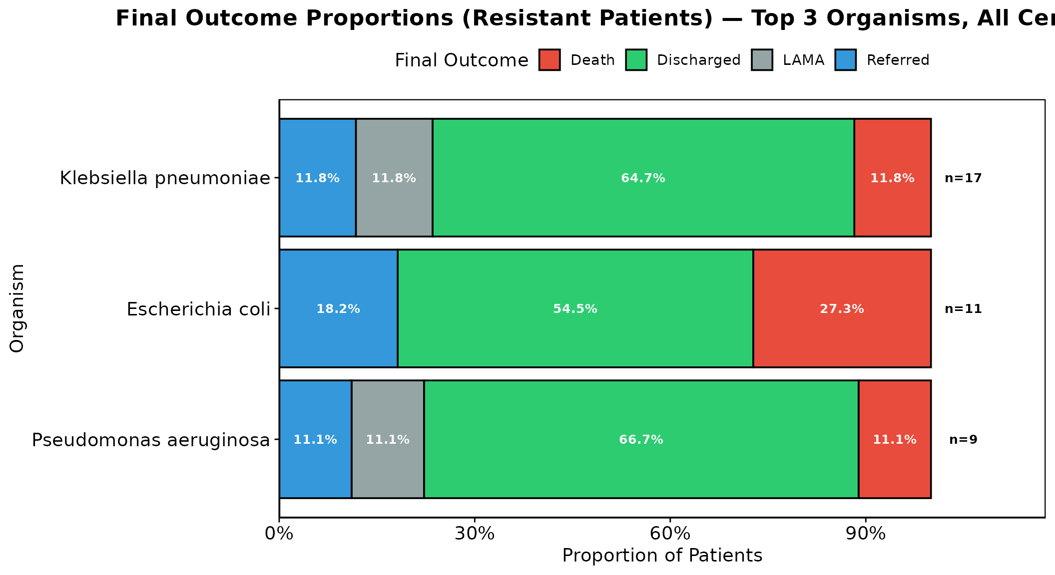
Outcome by organism, split by resistance status

resistance_filter = "R" shows patients with at least one R result for that organism; "S" shows patients with only S results. Because these groups overlap, calling the function once for each gives the fuller picture.

plot_outcome_by_organism(
  eda_data, n = 3, resistance_filter = "R", mode = "overall",
  patient_col = "patient_id", organism_col = "organism_normalized",
  antibiotic_col = "antibiotic_normalized", value_col = "ast_value_harmonized",
  outcome_col = "final_outcome", center_col = "center_name"
)

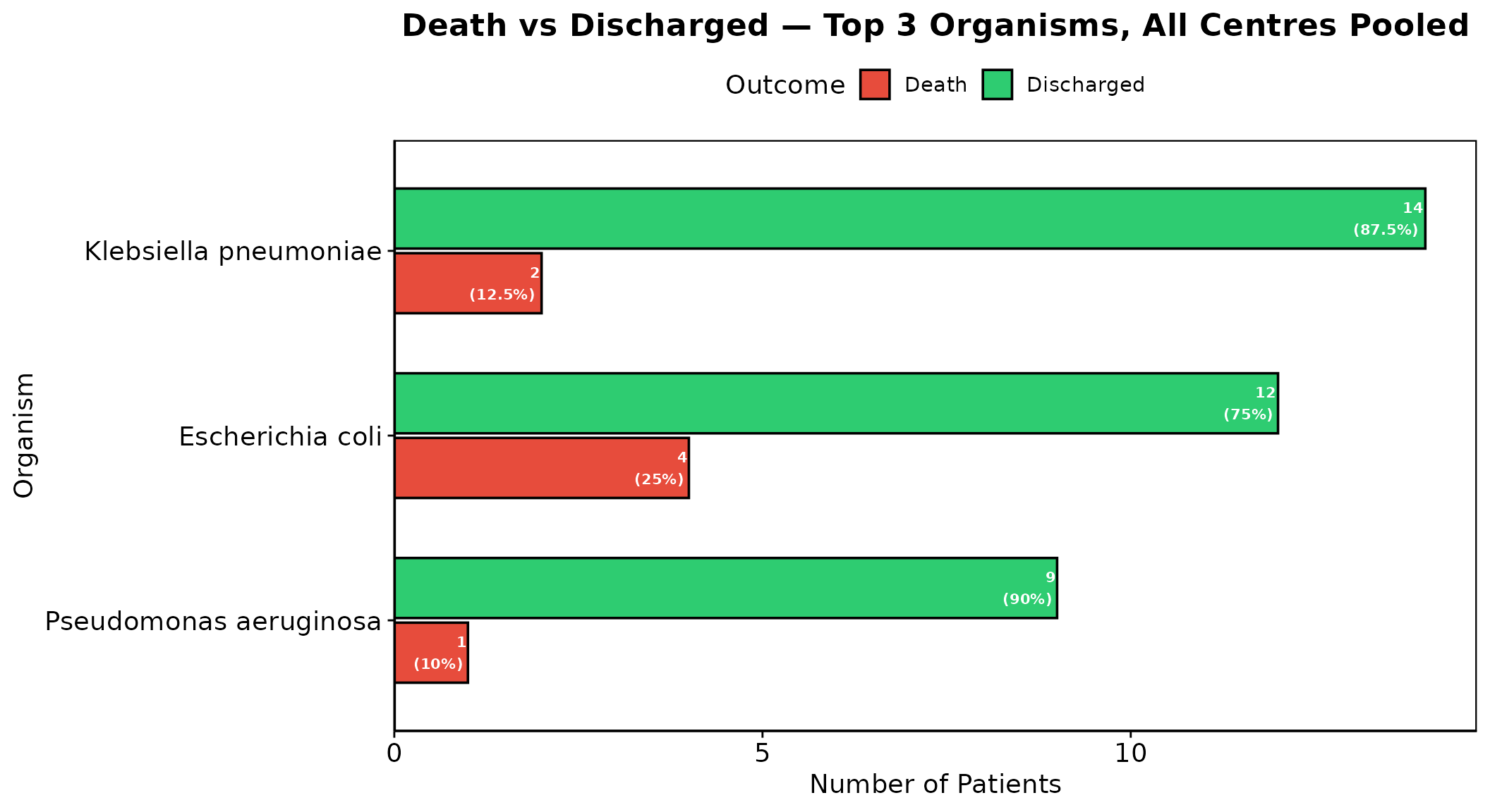
Death vs. discharged

plot_death_discharged(
  eda_data, n = 3, mode = "overall",
  patient_col = "patient_id", organism_col = "organism_normalized",
  outcome_col = "final_outcome", center_col = "center_name",
  antibiotic_col = "antibiotic_normalized", value_col = "ast_value_harmonized"
)

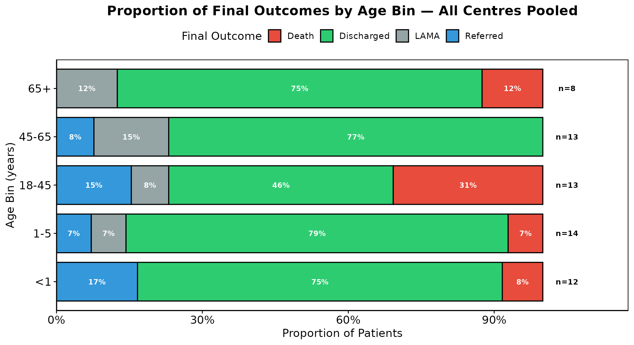
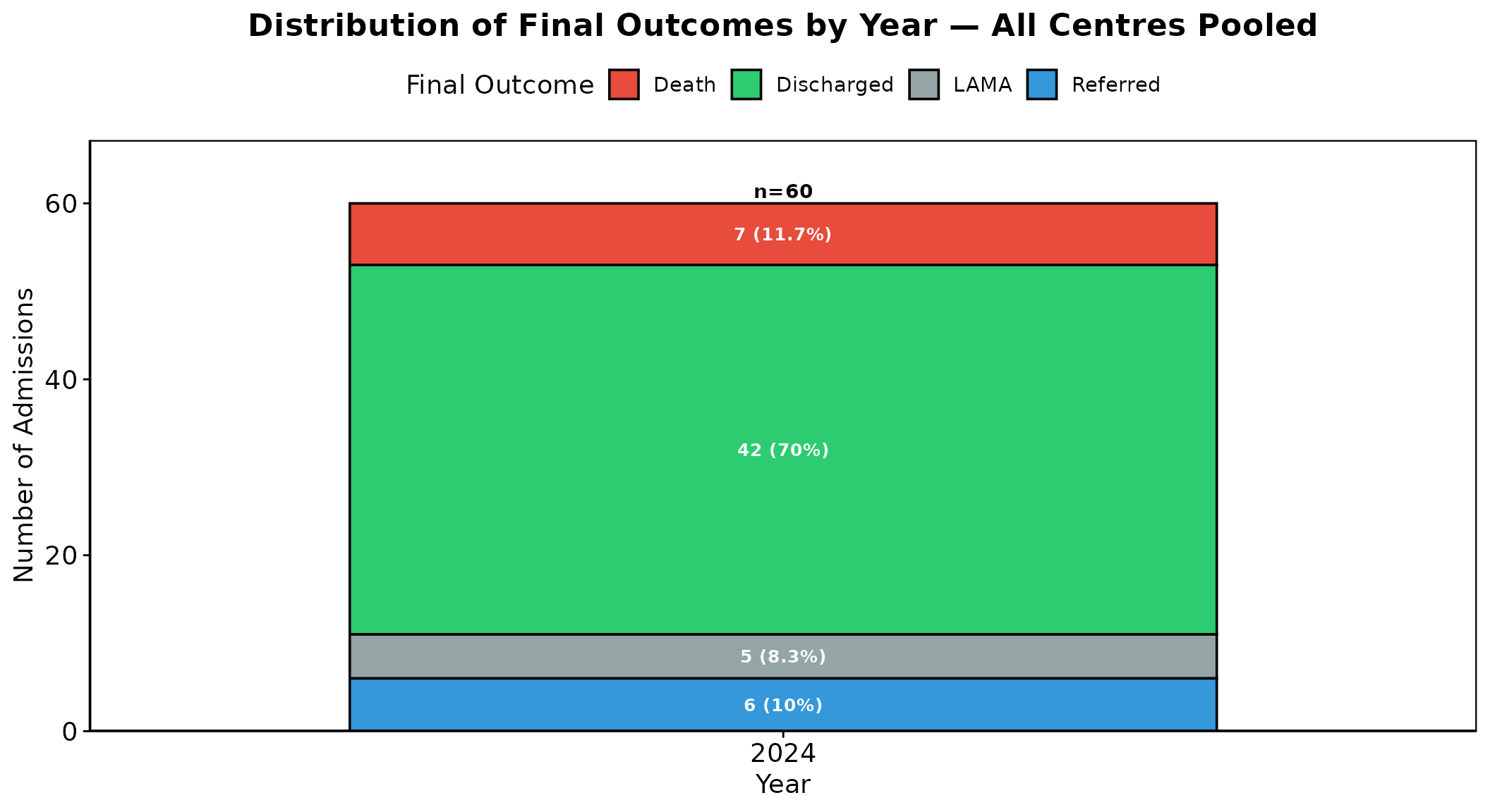
Outcome by age bin and by year

plot_outcome_by_agebin(
  eda_data, mode = "overall",
  patient_col = "patient_id", agebin_col = "Age_bin",
  outcome_col = "final_outcome", center_col = "center_name"
)

plot_outcome_by_year(
  eda_data, mode = "overall",
  patient_col = "patient_id", outcome_col = "final_outcome",
  date_col = "date_of_final_outcome", center_col = "center_name"
)

Case-Mix and Facility Patterns

Patients per hospital

plot_patients_by_hospital(eda_data, patient_col = "patient_id", center_col = "center_name")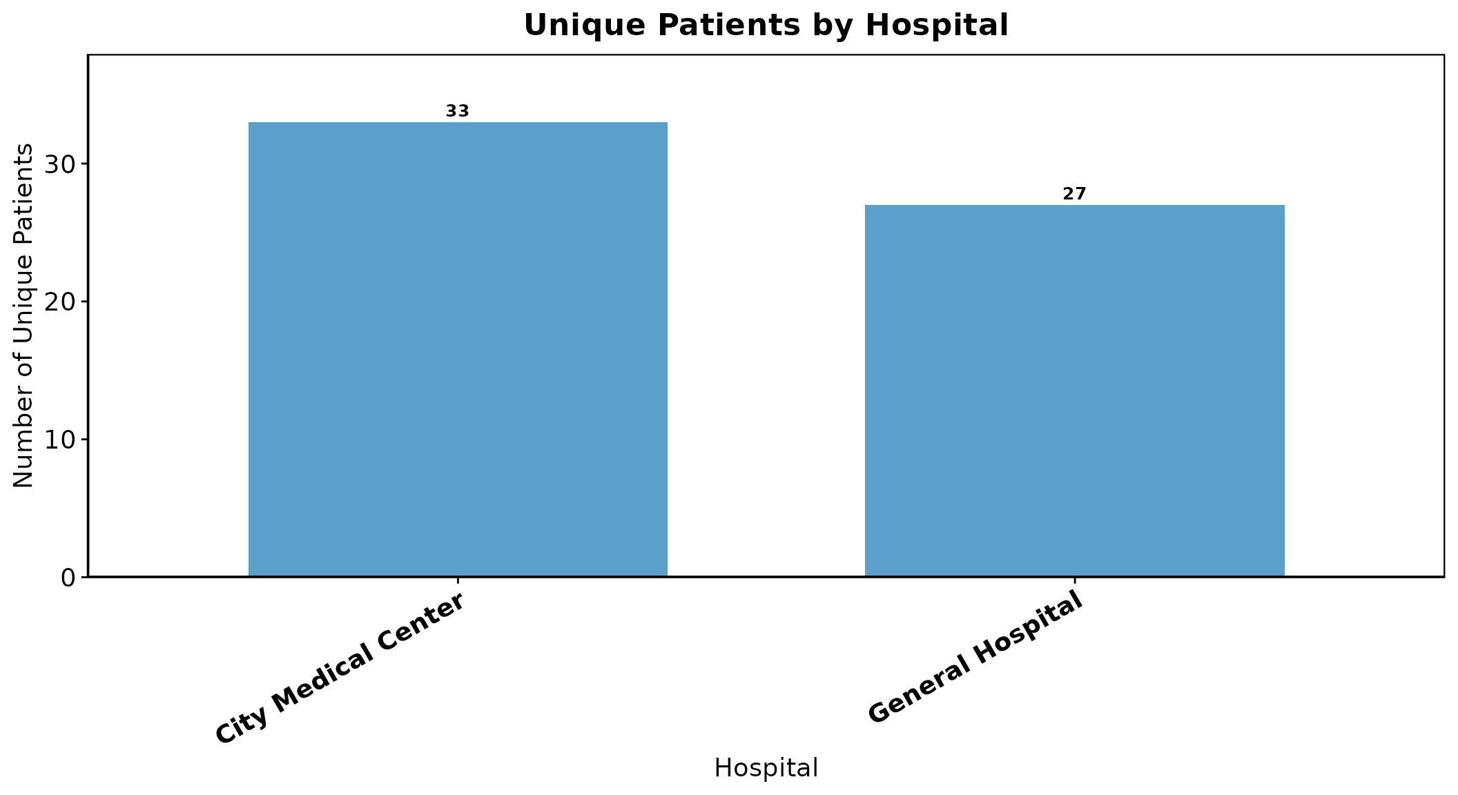

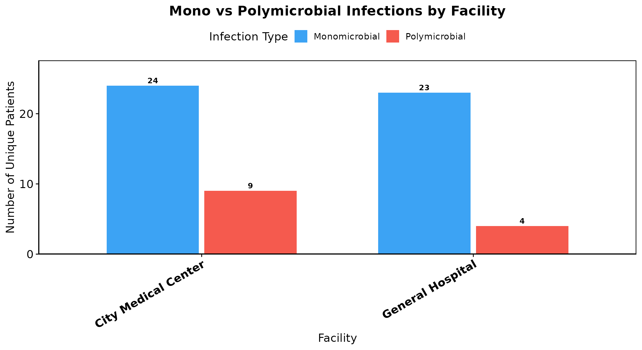
Monomicrobial vs. polymicrobial, by facility

plot_mono_poly_by_facility(
  eda_data, patient_col = "patient_id", poly_col = "is_polymicrobial", center_col = "center_name"
)

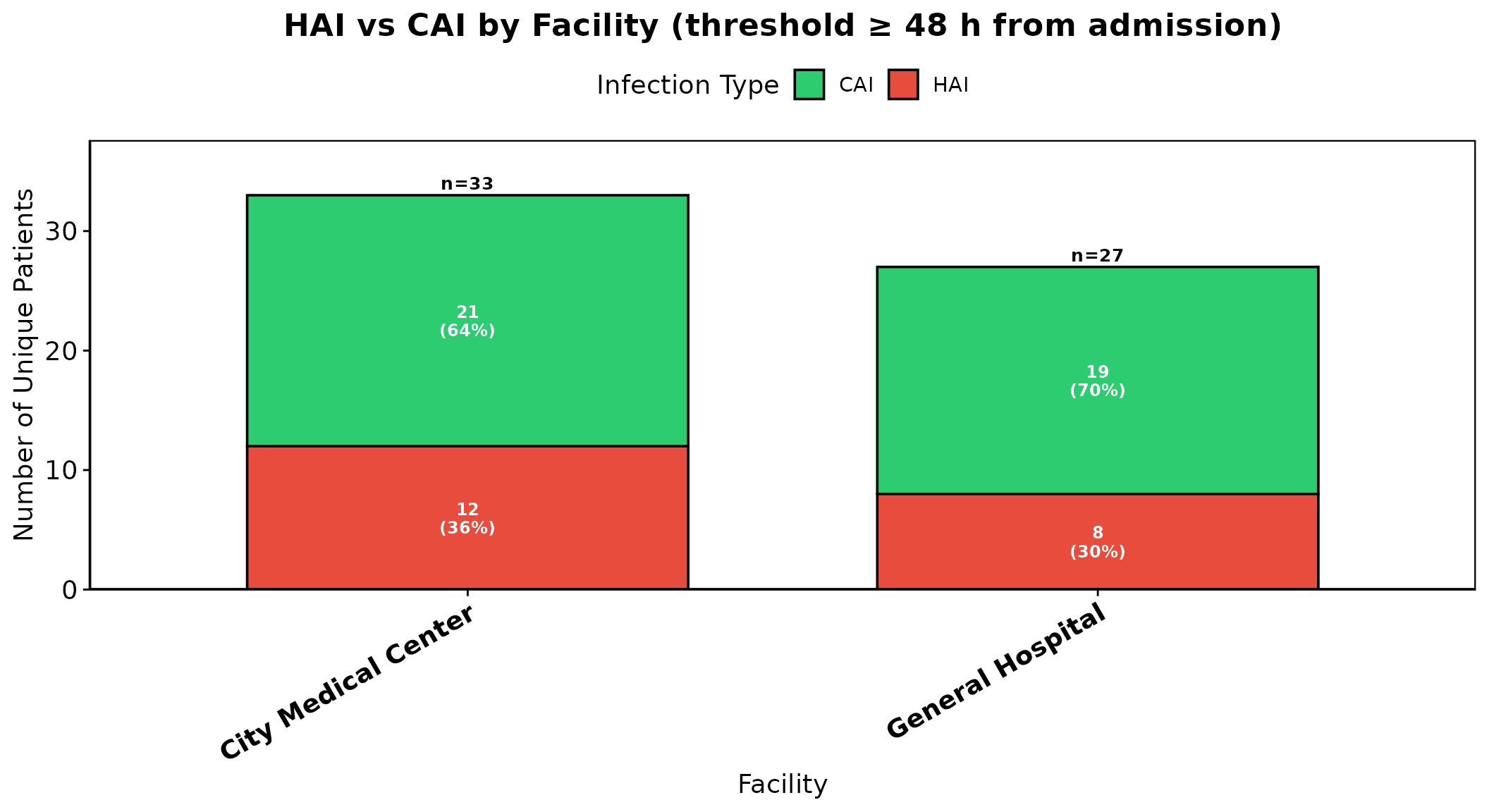
HAI vs. CAI, by facility

Computed from the gap between admission_col and culture_col, using hai_threshold_hours (default 48h) when an explicit infection-type column is not already available.

plot_hai_cai_by_facility(
  eda_data, patient_col = "patient_id", center_col = "center_name",
  admission_col = "date_of_admission", culture_col = "date_of_culture"
)

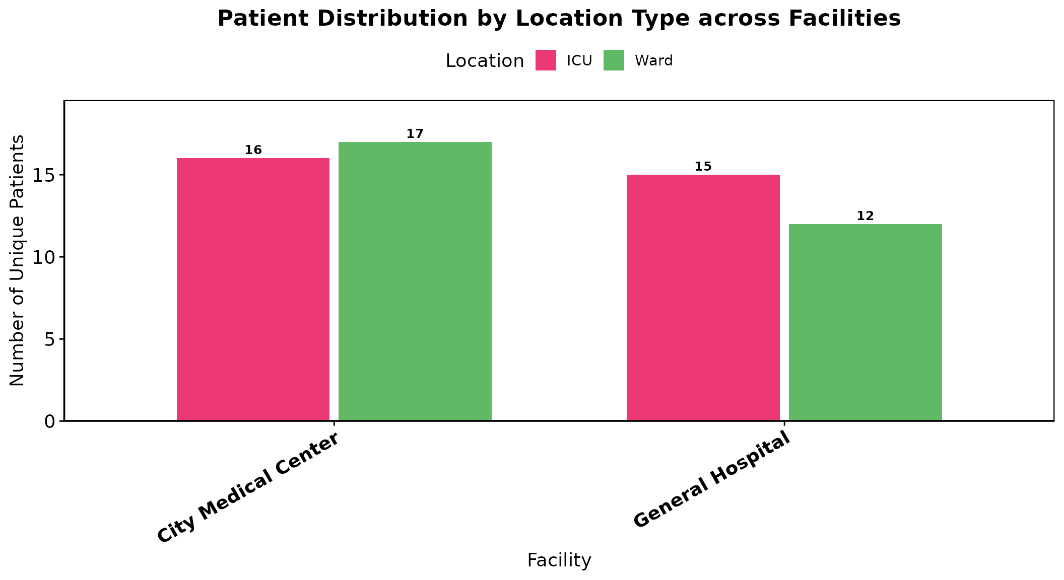
Location (ICU vs. Ward), by facility

plot_location_by_facility(
  eda_data, patient_col = "patient_id", location_col = "location", center_col = "center_name"
)

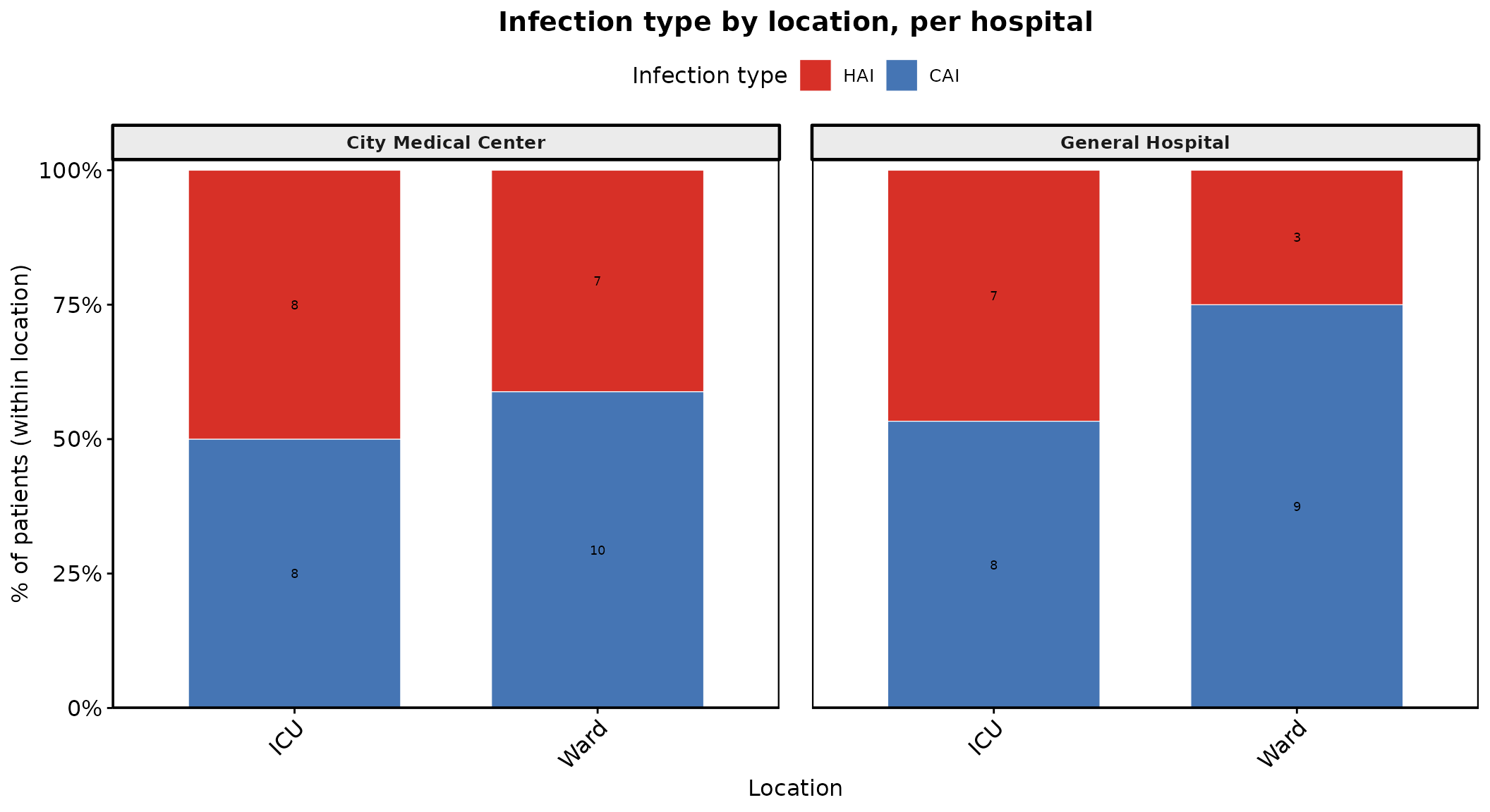
Infection type by location

plot_infection_type_by_location(
  eda_data, style = "bar", patient_col = "patient_id", center_col = "center_name",
  location_col = "location", infection_col = "infection_type"
)

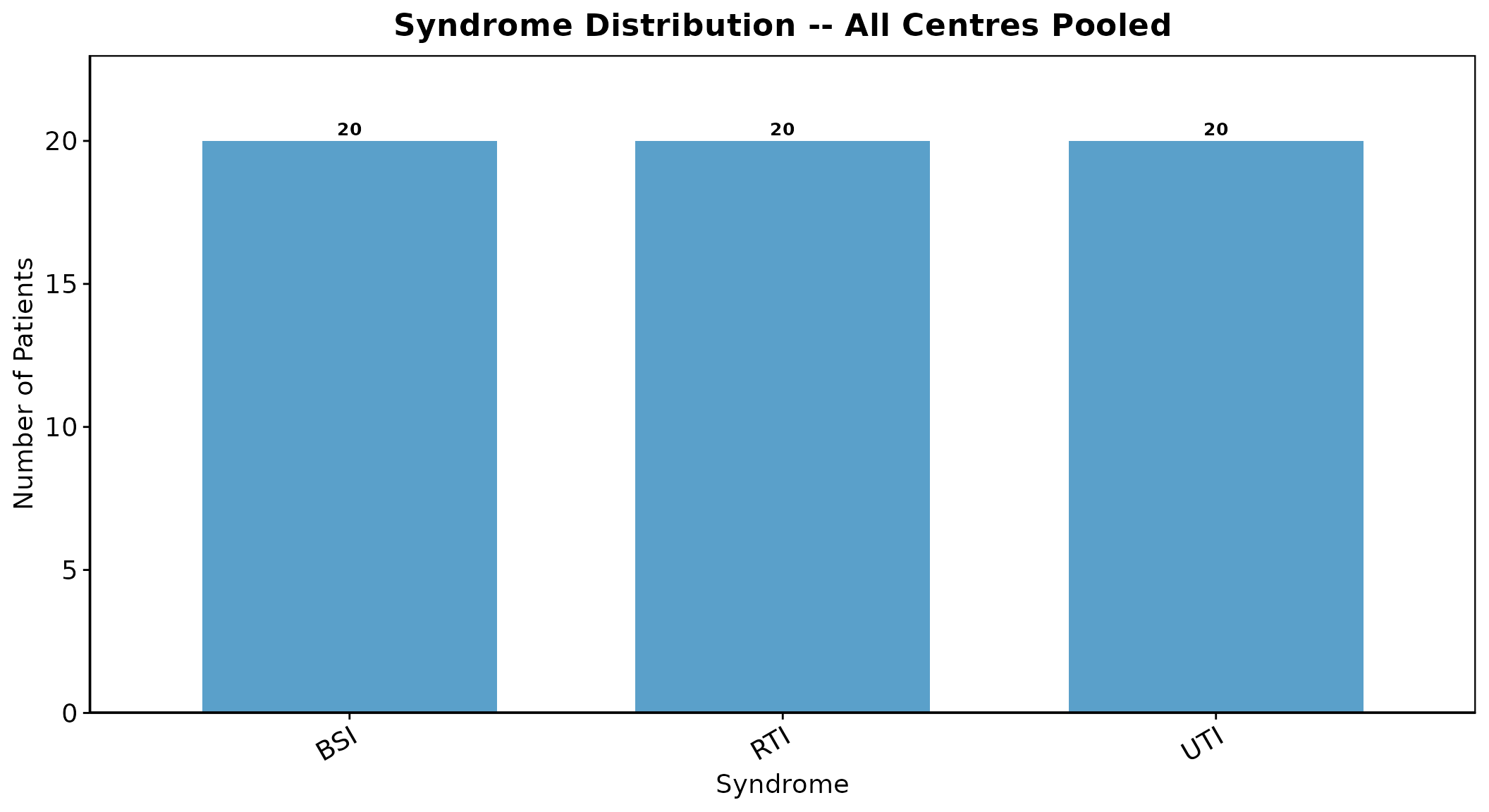
Syndrome distribution

plot_syndrome_distribution(
  eda_data, mode = "overall", patient_col = "patient_id",
  syndrome_col = "infectious_syndrome", center_col = "center_name"
)

Length of Stay and Age Distributions

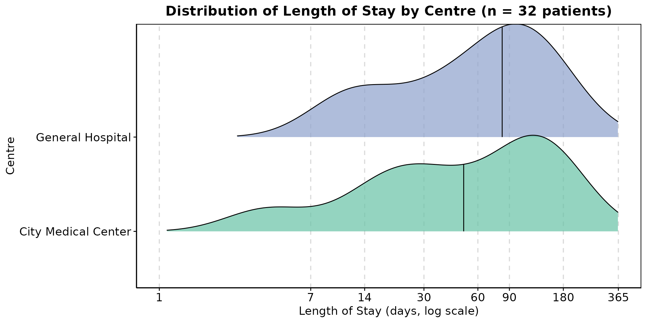
LOS ridge plot

plot_los_ridge(
  eda_data, mode = "all", patient_col = "patient_id", center_col = "center_name",
  admission_col = "date_of_admission", discharge_col = "date_of_final_outcome"
)

Age ridge plot

plot_age_ridge(eda_data, mode = "all", patient_col = "patient_id", age_col = "Age", center_col = "center_name")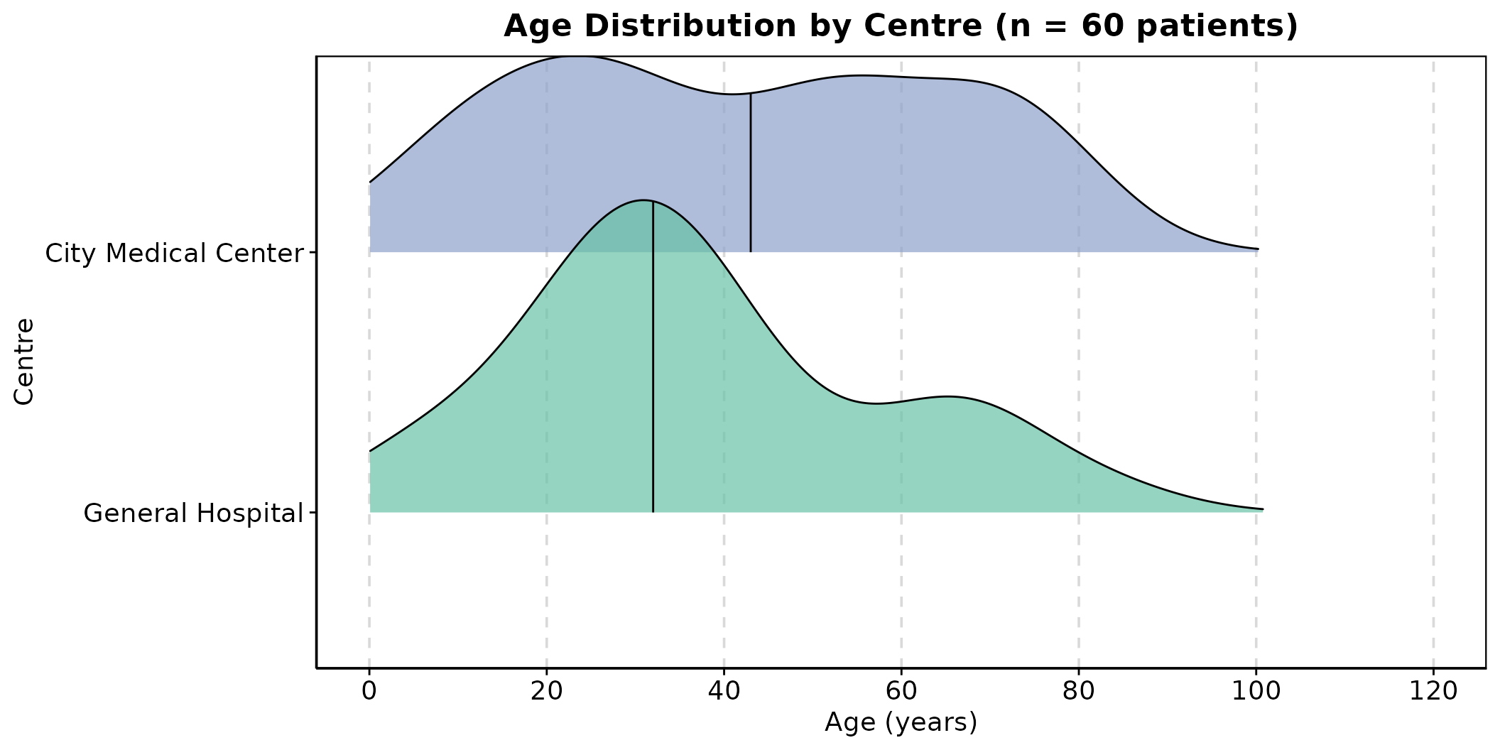

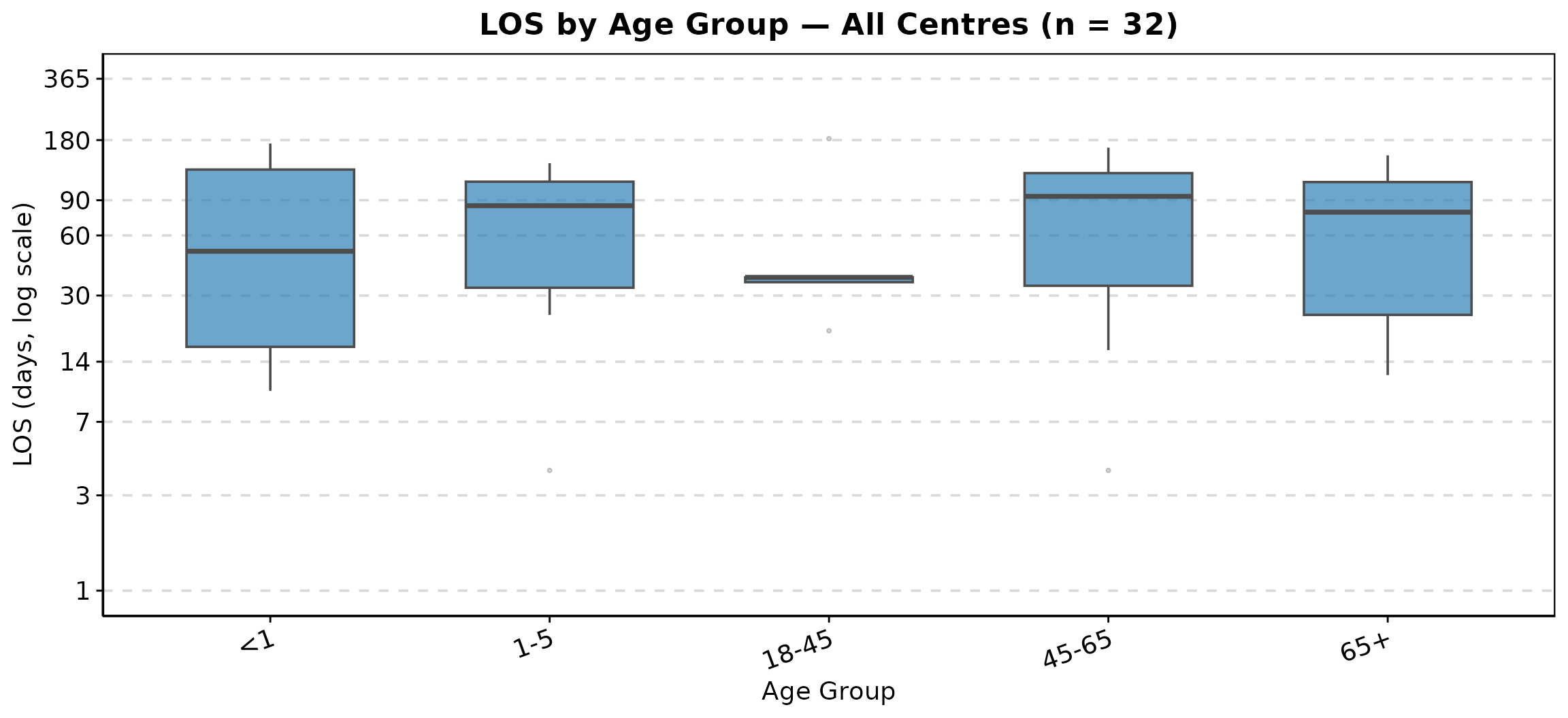
LOS by age bin

plot_los_by_agebin(
  eda_data, mode = "overall", patient_col = "patient_id", agebin_col = "Age_bin",
  age_col = "Age", center_col = "center_name",
  admission_col = "date_of_admission", discharge_col = "date_of_final_outcome"
)

Pipeline at a Glance

Preprocessing output (prep_* pipeline, analysis-ready long-format data)
          │
          ▼
  plot_top_organisms() / plot_abx_susceptibility() / plot_abx_heatmap()
  plot_resistance_by_sample() / plot_resistance_by_agebin() / plot_resistance_by_organism()
          │            (organism & susceptibility overview)
          ▼
  plot_outcome_distribution() / plot_outcome_by_organism() / plot_death_discharged()
  plot_outcome_by_agebin() / plot_outcome_by_year()
          │            (outcome patterns)
          ▼
  plot_patients_by_hospital() / plot_mono_poly_by_facility() / plot_hai_cai_by_facility()
  plot_location_by_facility() / plot_infection_type_by_location() / plot_syndrome_distribution()
          │            (case-mix and facility patterns)
          ▼
  plot_los_ridge() / plot_age_ridge() / plot_los_by_agebin()
          │            (LOS / age distributions)
          ▼
  Reviewed cohort -> proceed to DALY Burden Estimation (Pipeline 3)

Summary

The EDA layer is meant to be run interactively, plot by plot, while deciding whether the preprocessed cohort is ready for burden estimation – not wrapped into a single automated entry point the way run_preprocess() is for Pipeline 1. A typical review pass:

Check organism and susceptibility patterns for anything unexpected (plot_top_organisms(), plot_abx_heatmap())
Check outcome distributions and case-mix balance across centres
Check LOS/age distributions for implausible values before they reach burden estimation
Only then move on to the DALY Burden Estimation vignette

Session Info

sessionInfo()
#> R version 4.6.1 (2026-06-24)
#> Platform: x86_64-pc-linux-gnu
#> Running under: Ubuntu 24.04.4 LTS
#> 
#> Matrix products: default
#> BLAS:   /usr/lib/x86_64-linux-gnu/openblas-pthread/libblas.so.3 
#> LAPACK: /usr/lib/x86_64-linux-gnu/openblas-pthread/libopenblasp-r0.3.26.so;  LAPACK version 3.12.0
#> 
#> locale:
#>  [1] LC_CTYPE=C.UTF-8       LC_NUMERIC=C           LC_TIME=C.UTF-8       
#>  [4] LC_COLLATE=C.UTF-8     LC_MONETARY=C.UTF-8    LC_MESSAGES=C.UTF-8   
#>  [7] LC_PAPER=C.UTF-8       LC_NAME=C              LC_ADDRESS=C          
#> [10] LC_TELEPHONE=C         LC_MEASUREMENT=C.UTF-8 LC_IDENTIFICATION=C   
#> 
#> time zone: UTC
#> tzcode source: system (glibc)
#> 
#> attached base packages:
#> [1] stats     graphics  grDevices utils     datasets  methods   base     
#> 
#> other attached packages:
#> [1] dplyr_1.2.1        anumaan_0.1.0.9033
#> 
#> loaded via a namespace (and not attached):
#>  [1] janeaustenr_1.0.0  tidyr_1.3.2        sass_0.4.10        generics_0.1.4    
#>  [5] rstatix_1.1.0      stringi_1.8.9      lattice_0.22-9     digest_0.6.39     
#>  [9] magrittr_2.0.5     evaluate_1.0.5     grid_4.6.1         RColorBrewer_1.1-3
#> [13] fastmap_1.2.0      jsonlite_2.0.0     Matrix_1.7-5       tidytext_0.4.3    
#> [17] backports_1.5.1    Formula_1.2-6      purrr_1.2.2        scales_1.4.0      
#> [21] textshaping_1.0.5  jquerylib_0.1.4    abind_1.4-8        cli_3.6.6         
#> [25] rlang_1.3.0        tokenizers_0.3.0   withr_3.0.3        cachem_1.1.0      
#> [29] yaml_2.3.12        otel_0.2.0         tools_4.6.1        ggsignif_0.6.4    
#> [33] ggplot2_4.0.3      ggpubr_1.0.0       broom_1.0.13       vctrs_0.7.3       
#> [37] R6_2.6.1           ggridges_0.5.7     lifecycle_1.0.5    car_3.1-5         
#> [41] fs_2.1.0           ragg_1.5.2         pkgconfig_2.0.3    desc_1.4.3        
#> [45] pkgdown_2.2.1      pillar_1.11.1      bslib_0.12.0       gtable_0.3.6      
#> [49] glue_1.8.1         Rcpp_1.1.2         systemfonts_1.3.2  xfun_0.60         
#> [53] tibble_3.3.1       tidyselect_1.2.1   knitr_1.51         farver_2.1.2      
#> [57] htmltools_0.5.9    SnowballC_0.7.1    labeling_0.4.3     carData_3.0-6     
#> [61] rmarkdown_2.32     compiler_4.6.1     S7_0.2.2

Exploratory Data Analysis in anumaan

2026-09-04