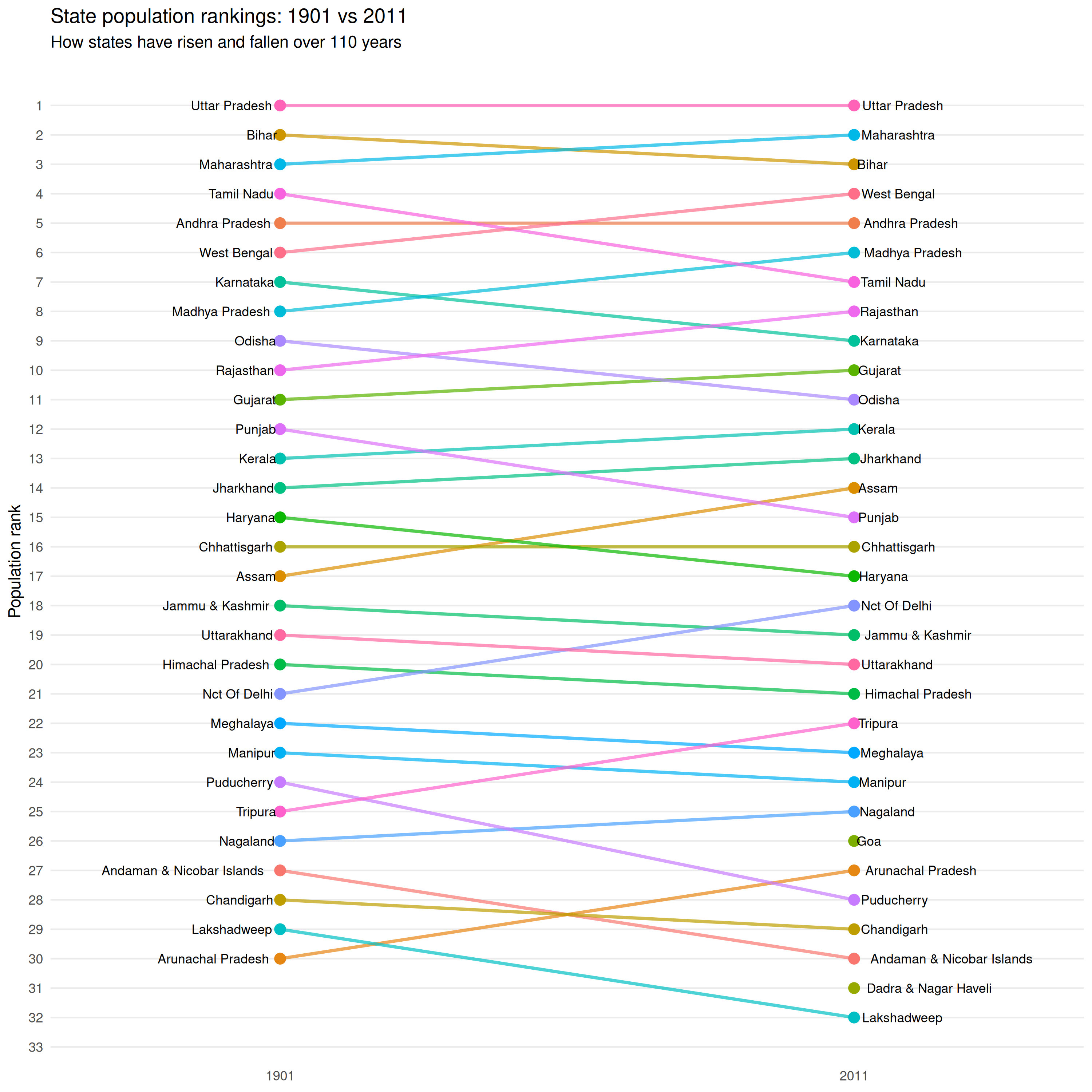
State ranking changes (1901-2011)
How have state populations shifted over 110 years?
rankings <- census_population_time_series |>
  filter(geography == "state", year %in% c(1901, 2011)) |>
  group_by(year) |>
  mutate(rank = rank(-population, ties.method = "first")) |>
  ungroup() |>
  select(year, state_name_harmonized, population, rank)

rank_change <- rankings |>
  pivot_wider(names_from = year, values_from = c(population, rank)) |>
  mutate(
    rank_change = rank_1901 - rank_2011,
    direction = case_when(
      rank_change > 0 ~ "Gained",
      rank_change < 0 ~ "Lost",
      TRUE ~ "Same"
    )
  )

ggplot(rankings, aes(x = factor(year), y = rank, group = state_name_harmonized)) +
  geom_line(aes(color = state_name_harmonized), linewidth = 1, alpha = 0.7) +
  geom_point(aes(color = state_name_harmonized), size = 3) +
  geom_text(
    data = filter(rankings, year == 1901),
    aes(label = state_name_harmonized),
    hjust = 1.1, size = 3
  ) +
  geom_text(
    data = filter(rankings, year == 2011),
    aes(label = state_name_harmonized),
    hjust = -0.1, size = 3
  ) +
  scale_y_reverse(breaks = 1:35) +
  scale_x_discrete(expand = expansion(mult = c(0.4, 0.4))) +
  labs(
    x = NULL,
    y = "Population rank",
    title = "State population rankings: 1901 vs 2011",
    subtitle = "How states have risen and fallen over 110 years"
  ) +
  theme_minimal() +
  theme(
    legend.position = "none",
    panel.grid.major.x = element_blank(),
    panel.grid.minor = element_blank()
  )
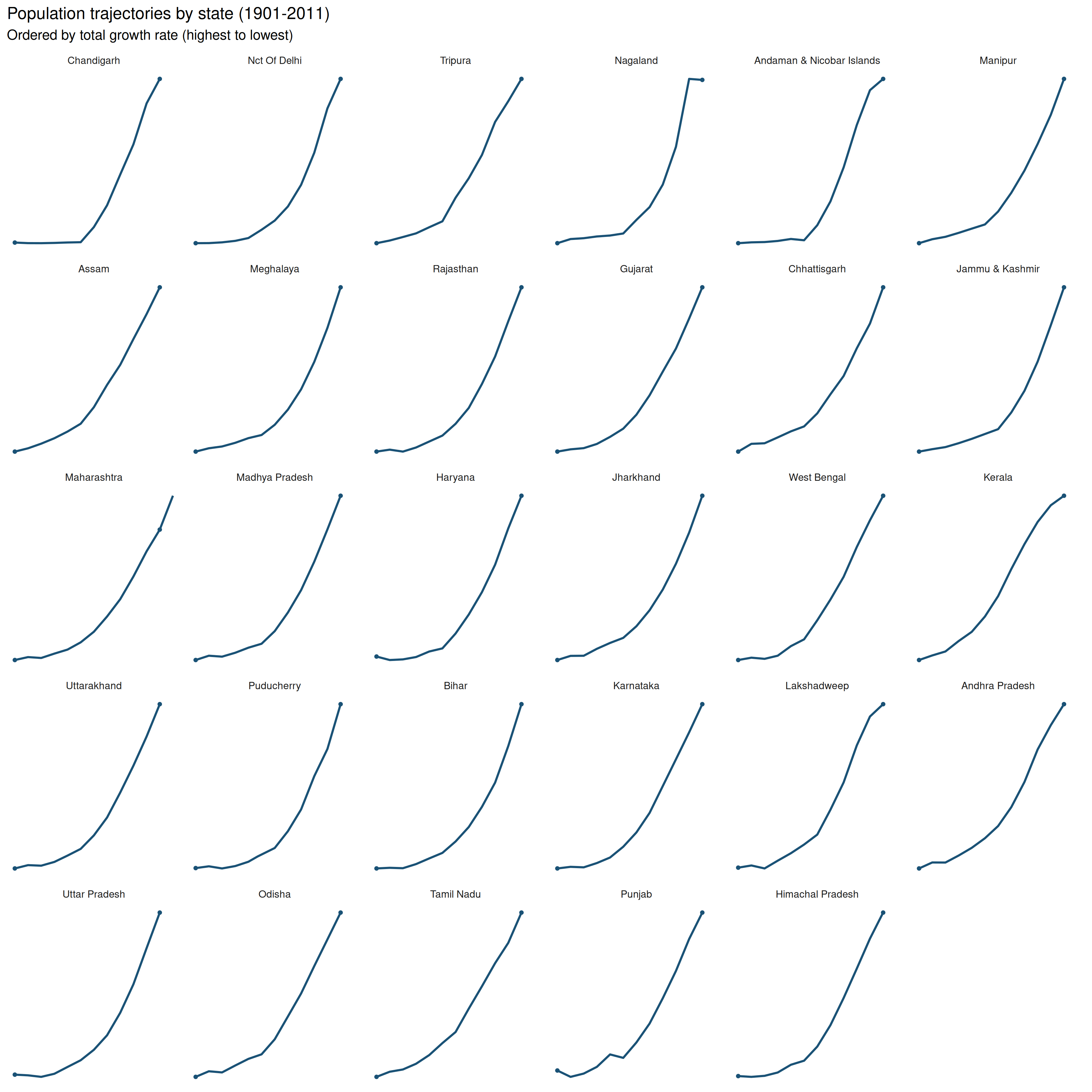
State population trajectories
state_trajectories <- census_population_time_series |>
  filter(geography == "state") |>
  group_by(state_name_harmonized) |>
  mutate(
    pop_scaled = (population - min(population, na.rm = TRUE)) /
      (max(population, na.rm = TRUE) - min(population, na.rm = TRUE))
  ) |>
  ungroup()

growth_order <- state_trajectories |>
  filter(year %in% c(1901, 2011)) |>
  group_by(state_name_harmonized) |>
  filter(n() == 2) |>
  summarise(
    growth = (population[year == 2011] / population[year == 1901]) - 1,
    .groups = "drop"
  ) |>
  filter(!is.na(growth)) |>
  arrange(desc(growth))

state_trajectories <- state_trajectories |>
  filter(state_name_harmonized %in% growth_order$state_name_harmonized) |>
  mutate(state_name_harmonized = factor(
    state_name_harmonized,
    levels = growth_order$state_name_harmonized
  ))

ggplot(state_trajectories, aes(year, pop_scaled)) +
  geom_line(color = "#1a5276", linewidth = 0.8) +
  geom_point(
    data = filter(state_trajectories, year %in% c(1901, 2011)),
    color = "#1a5276", size = 1
  ) +
  facet_wrap(~state_name_harmonized, ncol = 6) +
  labs(
    x = NULL, y = NULL,
    title = "Population trajectories by state (1901-2011)",
    subtitle = "Ordered by total growth rate (highest to lowest)"
  ) +
  theme_minimal() +
  theme(
    axis.text = element_blank(),
    panel.grid = element_blank(),
    strip.text = element_text(size = 8)
  )
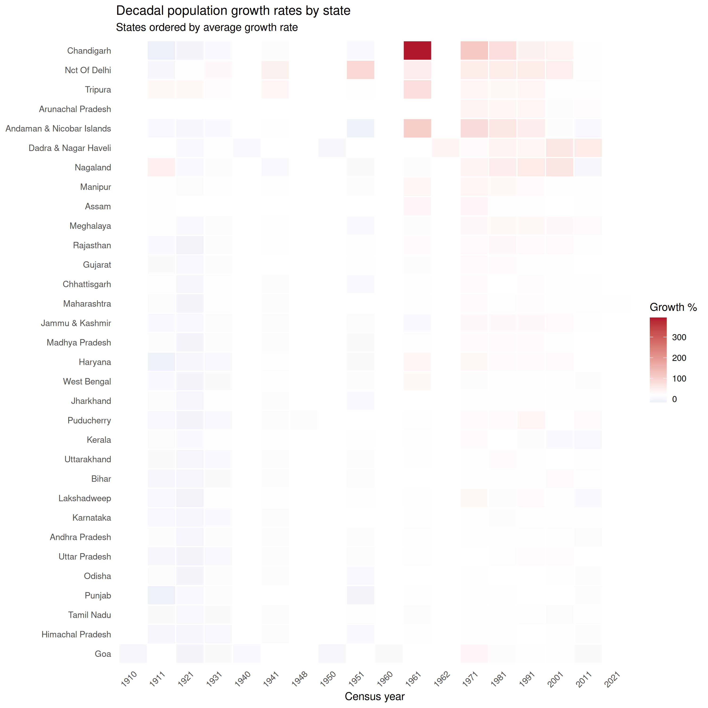
Decadal growth rates
growth_data <- census_population_time_series |>
  filter(geography == "state", !is.na(variation_percent)) |>
  select(year, state_name_harmonized, variation_percent)

# Order states by average growth
state_order <- growth_data |>
  group_by(state_name_harmonized) |>
  summarise(avg_growth = mean(variation_percent, na.rm = TRUE)) |>
  arrange(avg_growth) |>
  pull(state_name_harmonized)

growth_data <- growth_data |>
  mutate(state_name_harmonized = factor(state_name_harmonized, levels = state_order))

ggplot(growth_data, aes(factor(year), state_name_harmonized, fill = variation_percent)) +
  geom_tile(color = "white", linewidth = 0.5) +
  scale_fill_gradient2(
    low = "#2166ac", mid = "white", high = "#b2182b",
    midpoint = 20, na.value = "grey90",
    name = "Growth %"
  ) +
  labs(
    x = "Census year",
    y = NULL,
    title = "Decadal population growth rates by state",
    subtitle = "States ordered by average growth rate"
  ) +
  theme_minimal() +
  theme(
    axis.text.x = element_text(angle = 45, hjust = 1),
    panel.grid = element_blank()
  )