PM2.5 Regional Analysis
from vayuayan import PM25Client
import geopandas as gpd
import matplotlib.pyplot as plt
import pandas as pd
import json
1. Understanding PM2.5 Data
2. Initialize PM2.5 Client
# Initialize PM2.5 client
pm25_client = PM25Client()

print("PM2.5 Client initialized successfully")
PM2.5 Client initialized successfully
3. Downloading india states GeoJSON File
# Download and save the GeoJSON file for india states

sample_geojson = gpd.read_file(
    "https://gist.githubusercontent.com/JaggeryArray/fa31964eedb0c2da023c9485772f911a/raw/02c0644de34fbae9dbac2ba0496a00772a2c28cd/india_map_states.geojson"
)

# Save to file
geojson_file = "indian_states.geojson"
sample_geojson.to_file(geojson_file, driver="GeoJSON")
4. Visualize the GeoJSON Region
# Load and visualize the GeoJSON
gdf = gpd.read_file(geojson_file)

fig, ax = plt.subplots(figsize=(5, 5))
gdf.plot(ax=ax, facecolor="lightblue", edgecolor="black", linewidth=2)
ax.set_title("Analysis Region", fontsize=16, fontweight="bold")
ax.set_xlabel("Longitude")
ax.set_ylabel("Latitude")
plt.grid(True, alpha=0.3)
plt.tight_layout()
plt.show()

print("\nRegion Details:")
print(f"CRS: {gdf.crs}")
print(f"Number of Features: {len(gdf)}")
print(f"Columns: {gdf.columns.tolist()}")
print(f"Name: {gdf['state_name'].iloc[0]}")
print(f"Bounds: {gdf.total_bounds}")
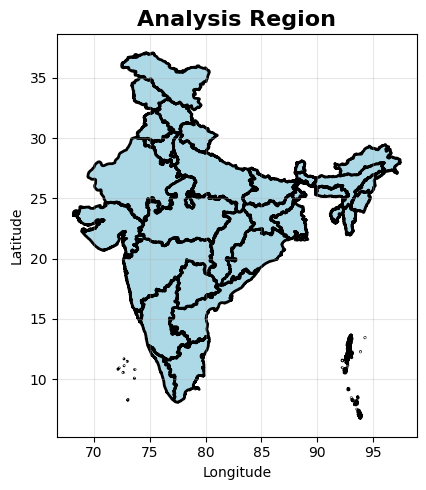
Region Details:
CRS: EPSG:4326
Number of Features: 36
Columns: ['state_name', 'state_code', 'geometry']
Name: A & N Islands
Bounds: [68.1776  6.7528 97.4129 37.0881]
5. Get PM2.5 Statistics for the complete India for 2023
# Get PM2.5 statistics for the region
# Specify year and optionally month

year = 2023
month = 2  # February (optional, leave as None for annual data)

try:
    stats = pm25_client.get_pm25_stats(geojson_file, year, month)

    print(f"PM2.5 Statistics for {year}/{month if month else 'Annual'}:")
    print(f"\nMean PM2.5: {stats['mean']:.2f} μg/m³")
    print(f"Standard Deviation: {stats['std']:.2f} μg/m³")
    print(f"Minimum PM2.5: {stats['min']:.2f} μg/m³")
    print(f"Maximum PM2.5: {stats['max']:.2f} μg/m³")

    # Interpret the results
    if stats["mean"] <= 12:
        category = "✅ Good (WHO guideline)"
    elif stats["mean"] <= 35.4:
        category = "🟢 Moderate"
    elif stats["mean"] <= 55.4:
        category = "🟡 Unhealthy for Sensitive Groups"
    elif stats["mean"] <= 150.4:
        category = "🟠 Unhealthy"
    elif stats["mean"] <= 250.4:
        category = "🔴 Very Unhealthy"
    else:
        category = "🆘 Hazardous"

    print(f"\nAir Quality Category: {category}")

except FileNotFoundError as e:
    print(f"Error: {e}")
    print("\nNote: This requires PM2.5 netCDF data files.")
    print("Download from: https://sites.wustl.edu/acag/datasets/surface-pm2-5/")
Using cached file: pm25_data\V6GL02.04.CNNPM25.GL.202302-202302.nc
PM2.5 Statistics for 2023/2:

Mean PM2.5: 44.21 μg/m³
Standard Deviation: 18.75 μg/m³
Minimum PM2.5: -23.80 μg/m³
Maximum PM2.5: 201.80 μg/m³

Air Quality Category: 🟡 Unhealthy for Sensitive Groups
6. Analyze Multiple Sub-Regions
# Get PM2.5 statistics for each polygon
try:
    results = pm25_client.get_pm25_stats(
        geojson_file, year=2023, month=2, group_by="state_name"
    )

    # Convert to DataFrame for better visualization
    df_results = pd.DataFrame(results)

    print("PM2.5 Statistics by State:")
    print(df_results[["state_name", "mean", "std", "min", "max", "count"]])

    # Find state with highest pollution
    worst_state = df_results.loc[df_results["mean"].idxmax()]
    print(f"\nMost Polluted State: {worst_state['state_name']}")
    print(f"Average PM2.5: {worst_state['mean']:.2f} μg/m³")

except FileNotFoundError as e:
    print(f"Error: {e}")
    print("Note: This requires PM2.5 netCDF data files.")
Using cached file: pm25_data\V6GL02.04.CNNPM25.GL.202302-202302.nc
PM2.5 Statistics by State:
state_name mean std min max count
0 A & N Islands 26.736076 4.642200 10.559565 39.279202 7850
1 Andhra Pradesh 37.747311 7.710774 -13.700000 71.428101 140227
2 Arunachal Pradesh 25.289986 9.757482 8.589810 64.743187 76882
3 Assam 56.700302 14.021981 19.789631 112.994400 72621
4 Bihar 86.183090 17.285084 38.057251 138.052094 86164
5 Chandigarh 53.463982 2.594560 47.528309 59.226231 138
6 Chhattisgarh 43.921875 8.193904 -6.100000 167.313705 119463
7 DNHDD 39.369610 6.282200 16.576408 68.297791 687
8 Delhi 101.283966 13.680910 68.632477 130.057159 1496
9 Goa 40.856464 3.682843 22.005735 57.911633 3333
10 Gujarat 35.799759 7.888505 -23.299999 201.796555 164206
11 Haryana 65.518333 10.105743 34.220348 112.012245 42354
12 Himachal Pradesh 26.042427 6.449605 13.867519 51.061626 54242
13 Jammu & Kashmir 23.887915 5.516273 16.301540 48.607197 53969
14 Jharkhand 57.459743 12.035691 4.850131 148.433945 72272
15 Karnataka 33.316776 6.794228 1.931893 61.043396 163381
16 Kerala 38.901890 6.960310 21.096498 65.156235 33080
17 Ladakh 12.886016 3.502312 6.227266 24.695324 167888
18 Lakshadweep 53.007759 11.728984 35.933651 86.120010 84
19 Madhya Pradesh 38.588871 6.851001 -23.799999 89.274773 276492
20 Maharashtra 41.017254 6.347002 -12.600000 93.932137 267457
21 Manipur 53.500233 8.297816 36.365082 81.965469 20422
22 Meghalaya 65.241524 8.914769 42.956116 95.102303 20767
23 Mizoram 50.792274 9.762743 30.887281 84.194534 19157
24 Nagaland 50.964497 7.544705 30.654783 69.798721 15492
25 Odisha 52.571457 8.520728 -13.700000 103.609283 136647
26 Puducherry 35.211349 5.520503 9.309538 50.891384 662
27 Punjab 58.513329 8.605981 30.373760 85.687485 48536
28 Rajasthan 43.161564 6.603865 -11.500000 78.570801 313169
29 Sikkim 45.016693 6.523999 35.235641 65.802200 6749
30 Tamil Nadu 34.017384 4.743386 7.917448 66.359886 109304
31 Telangana 38.979332 4.714859 14.016782 75.282829 96893
32 Tripura 89.022141 11.420099 61.198307 133.052338 9710
33 Uttar Pradesh 69.170586 12.930211 15.006321 128.973419 222299
34 Uttarakhand 35.294258 10.839684 15.523481 81.931000 50939
35 West Bengal 82.156898 16.278830 10.066559 149.227112 78483
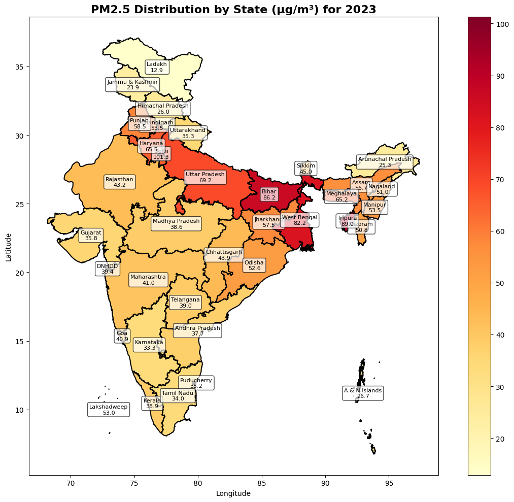
Most Polluted State: Delhi
Average PM2.5: 101.28 μg/m³
7. Visualize PM2.5 Distribution
# Load the multi-region GeoJSON
gdf_multi = gpd.read_file(geojson_file)

# Merge with results if available
try:
    # Merge PM2.5 data with geodataframe
    gdf_with_pm25 = gdf_multi.merge(
        df_results[["state_name", "mean"]],
        left_on="state_name",
        right_on="state_name",
    )

    # Create choropleth map
    fig, ax = plt.subplots(figsize=(12, 10))
    gdf_with_pm25.plot(
        column="mean",
        ax=ax,
        legend=True,
        cmap="YlOrRd",
        edgecolor="black",
        linewidth=1.5,
    )

    # Add district labels
    for idx, row in gdf_with_pm25.iterrows():
        centroid = row.geometry.centroid
        ax.text(
            centroid.x,
            centroid.y,
            f"{row['state_name']}\n{row['mean']:.1f}",
            ha="center",
            va="center",
            fontsize=8,
            bbox=dict(boxstyle="round", facecolor="white", alpha=0.7),
        )

    ax.set_title(
        "PM2.5 Distribution by State (μg/m³) for 2023", fontsize=16, fontweight="bold"
    )
    ax.set_xlabel("Longitude")
    ax.set_ylabel("Latitude")
    plt.tight_layout()
    plt.show()

except NameError:
    print("PM2.5 data not available. Run the previous cell first.")
8. Temporal Analysis
# Analyze PM2.5 for multiple months
months = range(1, 13)  # All 12 months
monthly_data = []

print("Analyzing monthly PM2.5 levels...\n")

for month in months:
    try:
        stats = pm25_client.get_pm25_stats(geojson_file, 2023, month)
        monthly_data.append(
            {
                "Month": month,
                "Mean_PM25": stats["mean"],
                "Std_PM25": stats["std"],
            }
        )
        print(f"Month {month}: {stats['mean']:.2f} μg/m³")
    except Exception as e:
        print(f"Month {month}: Data not available : {e}")

if monthly_data:
    # Create DataFrame
    df_monthly = pd.DataFrame(monthly_data)

    # Plot monthly trends
    plt.figure(figsize=(14, 6))
    plt.plot(
        df_monthly["Month"],
        df_monthly["Mean_PM25"],
        marker="o",
        linewidth=2,
        markersize=8,
    )
    plt.fill_between(
        df_monthly["Month"],
        df_monthly["Mean_PM25"] - df_monthly["Std_PM25"],
        df_monthly["Mean_PM25"] + df_monthly["Std_PM25"],
        alpha=0.3,
    )
    plt.xlabel("Month", fontsize=12)
    plt.ylabel("PM2.5 (μg/m³)", fontsize=12)
    plt.title("Monthly PM2.5 Trends", fontsize=14, fontweight="bold")
    plt.grid(True, alpha=0.3)
    plt.xticks(range(1, 13))
    plt.tight_layout()
    plt.show()

    # Find worst and best months
    worst_month = df_monthly.loc[df_monthly["Mean_PM25"].idxmax()]
    best_month = df_monthly.loc[df_monthly["Mean_PM25"].idxmin()]

    print(
        f"\nWorst Month: {worst_month['Month']} ({worst_month['Mean_PM25']:.2f} μg/m³)"
    )
    print(f"Best Month: {best_month['Month']} ({best_month['Mean_PM25']:.2f} μg/m³)")
Analyzing monthly PM2.5 levels...

Using cached file: pm25_data\V6GL02.04.CNNPM25.GL.202301-202301.nc
Month 1: Data not available : [Errno -101] NetCDF: HDF error: 'c:\\Users\\mahes\\OneDrive\\Desktop\\Coding\\DH307\\vayuayan\\docs\\notebooks\\pm25_data\\V6GL02.04.CNNPM25.GL.202301-202301.nc'
Using cached file: pm25_data\V6GL02.04.CNNPM25.GL.202302-202302.nc
Month 2: 44.21 μg/m³
Using cached file: pm25_data\V6GL02.04.CNNPM25.GL.202303-202303.nc
Month 3: 38.77 μg/m³
Using cached file: pm25_data\V6GL02.04.CNNPM25.GL.202304-202304.nc
Month 4: 33.03 μg/m³
Using cached file: pm25_data\V6GL02.04.CNNPM25.GL.202305-202305.nc
Month 5: 30.89 μg/m³
Using cached file: pm25_data\V6GL02.04.CNNPM25.GL.202306-202306.nc
Month 6: 28.29 μg/m³
Using cached file: pm25_data\V6GL02.04.CNNPM25.GL.202307-202307.nc
Month 7: 28.57 μg/m³
Using cached file: pm25_data\V6GL02.04.CNNPM25.GL.202308-202308.nc
Month 8: 31.72 μg/m³
Using cached file: pm25_data\V6GL02.04.CNNPM25.GL.202309-202309.nc
Month 9: 27.58 μg/m³
Using cached file: pm25_data\V6GL02.04.CNNPM25.GL.202310-202310.nc
Month 10: 40.79 μg/m³
Using cached file: pm25_data\V6GL02.04.CNNPM25.GL.202311-202311.nc
Month 11: 60.28 μg/m³
Using cached file: pm25_data\V6GL02.04.CNNPM25.GL.202312-202312.nc
Month 12: 58.04 μg/m³
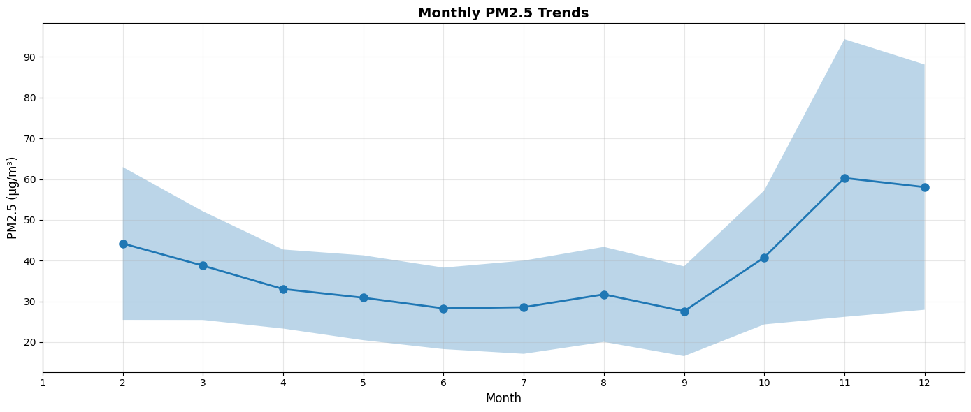
Worst Month: 11.0 (60.28 μg/m³)
Best Month: 9.0 (27.58 μg/m³)
9. Export Results
# Export results to CSV
if "df_results" in locals():
    output_file = "pm25_analysis_results.csv"
    df_results.to_csv(output_file, index=False)
    print(f"State-level results saved to: {output_file}")

if "df_monthly" in locals():
    monthly_output = "pm25_monthly_trends.csv"
    df_monthly.to_csv(monthly_output, index=False)
    print(f"Monthly trends saved to: {monthly_output}")
State-level results saved to: pm25_analysis_results.csv
Monthly trends saved to: pm25_monthly_trends.csv