Social composition

library(censusindia)
library(dplyr)
library(ggplot2)
library(ggtern)
library(ggridges)
library(patchwork)

SC/ST/General composition

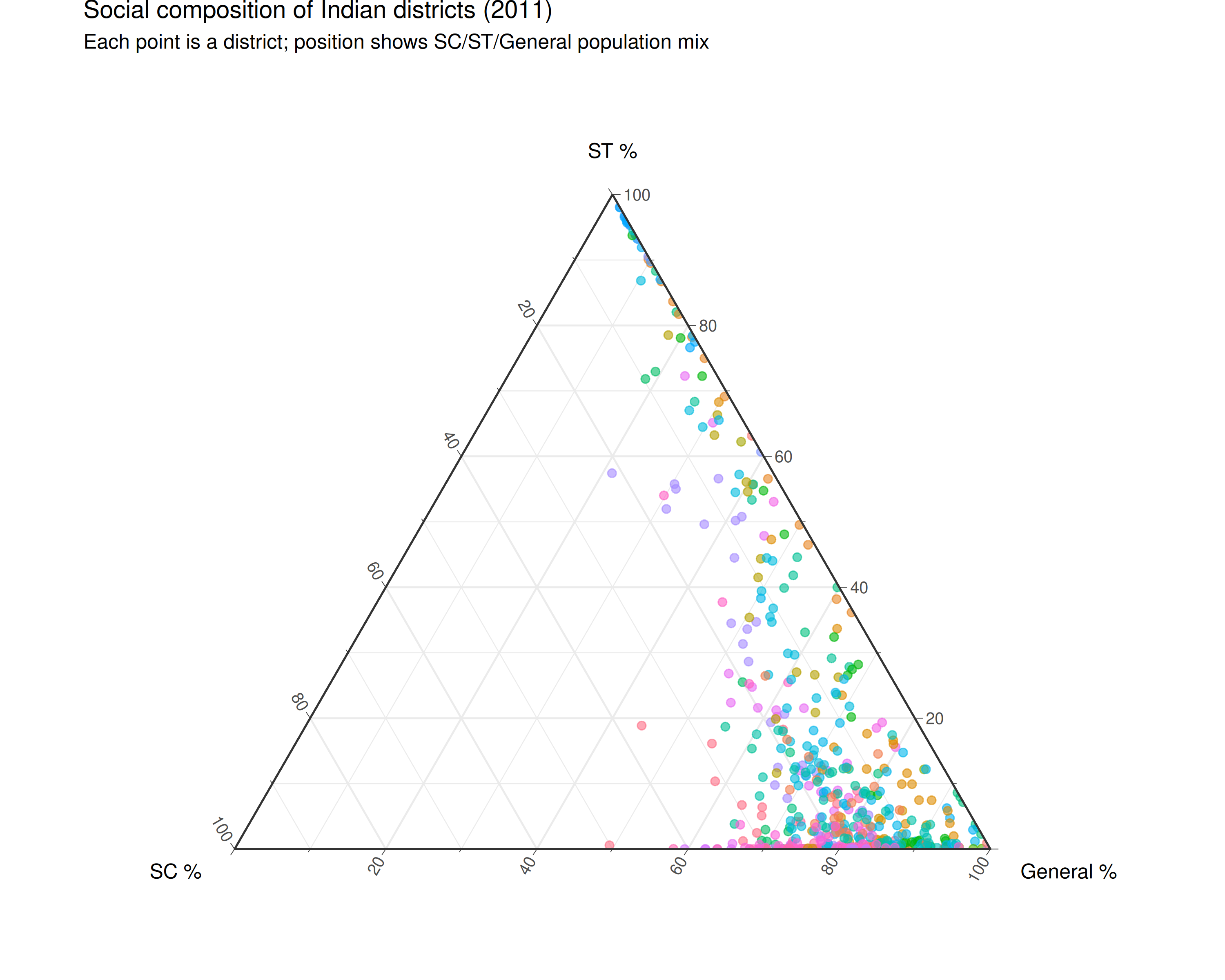
Each district has a different mix of Scheduled Caste, Scheduled Tribe, and general population. Ternary plots show these three-way proportions at a glance.

composition <- census_2011_pca |>
  filter(geography == "district") |>
  mutate(
    sc_pct = 100 * sc_population / population_total,
    st_pct = 100 * st_population / population_total,
    general_pct = 100 - sc_pct - st_pct
  ) |>
  filter(!is.na(sc_pct), !is.na(st_pct), general_pct >= 0)

ggtern(composition, aes(x = sc_pct, y = st_pct, z = general_pct)) +
  geom_point(aes(color = state_name_harmonized), alpha = 0.6, size = 2) +
  labs(
    x = "SC %",
    y = "ST %",
    z = "General %",
    title = "Social composition of Indian districts (2011)",
    subtitle = "Each point is a district; position shows SC/ST/General population mix"
  ) +
  theme_bw() +
  theme(
    legend.position = "none",
    ggtern.panel.background = element_rect(fill = "white")
  )

Regional patterns

regions <- tibble::tribble(
  ~state_name_harmonized, ~region,
  "Jammu & Kashmir", "North",
  "Himachal Pradesh", "North",
  "Punjab", "North",
  "Chandigarh", "North",
  "Uttarakhand", "North",
  "Haryana", "North",
  "Nct Of Delhi", "North",
  "Rajasthan", "North",
  "Uttar Pradesh", "North",
  "Bihar", "East",
  "West Bengal", "East",
  "Jharkhand", "East",
  "Odisha", "East",
  "Sikkim", "Northeast",
  "Arunachal Pradesh", "Northeast",
  "Nagaland", "Northeast",
  "Manipur", "Northeast",
  "Mizoram", "Northeast",
  "Tripura", "Northeast",
  "Meghalaya", "Northeast",
  "Assam", "Northeast",
  "Chhattisgarh", "Central",
  "Madhya Pradesh", "Central",
  "Gujarat", "West",
  "Daman & Diu", "West",
  "Dadra & Nagar Haveli", "West",
  "Maharashtra", "West",
  "Goa", "West",
  "Andhra Pradesh", "South",
  "Karnataka", "South",
  "Kerala", "South",
  "Tamil Nadu", "South",
  "Puducherry", "South",
  "Lakshadweep", "South",
  "Andaman & Nicobar Islands", "Islands",
  "Telangana", "South"
)

region_colors <- c(
  "North" = "#e63946",
  "East" = "#f4a261",
  "Northeast" = "#2a9d8f",
  "Central" = "#8338ec",
  "West" = "#3a86ff",
  "South" = "#06d6a0",
  "Islands" = "#adb5bd"
)

composition_region <- composition |>
  left_join(regions, by = "state_name_harmonized") |>
  filter(!is.na(region))

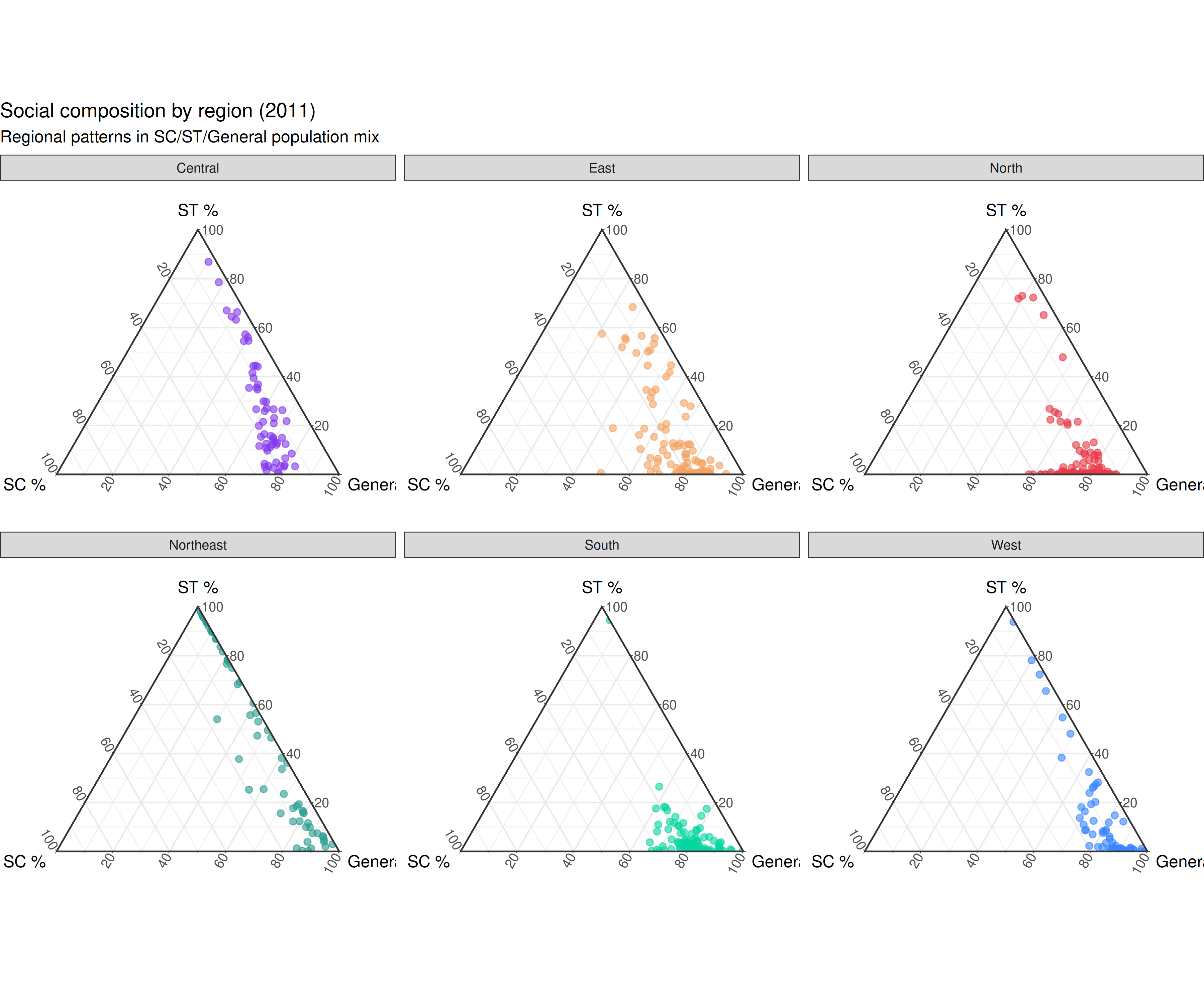
ggtern(composition_region, aes(x = sc_pct, y = st_pct, z = general_pct)) +
  geom_point(aes(color = region), alpha = 0.6, size = 2) +
  facet_wrap(~region, ncol = 3) +
  scale_color_manual(values = region_colors) +
  labs(
    x = "SC %",
    y = "ST %",
    z = "General %",
    title = "Social composition by region (2011)",
    subtitle = "Regional patterns in SC/ST/General population mix"
  ) +
  theme_bw() +
  theme(
    legend.position = "none",
    ggtern.panel.background = element_rect(fill = "white")
  )

SC population distribution by state

state_order <- composition |>
  group_by(state_name_harmonized) |>
  summarise(median_sc = median(sc_pct, na.rm = TRUE)) |>
  arrange(median_sc) |>
  pull(state_name_harmonized)

composition |>
  filter(state_name_harmonized %in% state_order) |>
  mutate(state_name_harmonized = factor(state_name_harmonized, levels = state_order)) |>
  ggplot(aes(x = sc_pct, y = state_name_harmonized, fill = stat(x))) +
  geom_density_ridges_gradient(scale = 2, rel_min_height = 0.01) +
  scale_fill_gradient(low = "#fce4ec", high = "#880e4f", name = "SC %") +
  labs(
    x = "SC population (%)",
    y = NULL,
    title = "Distribution of SC population across districts",
    subtitle = "States ordered by median SC percentage"
  ) +
  theme_minimal() +
  theme(legend.position = "right")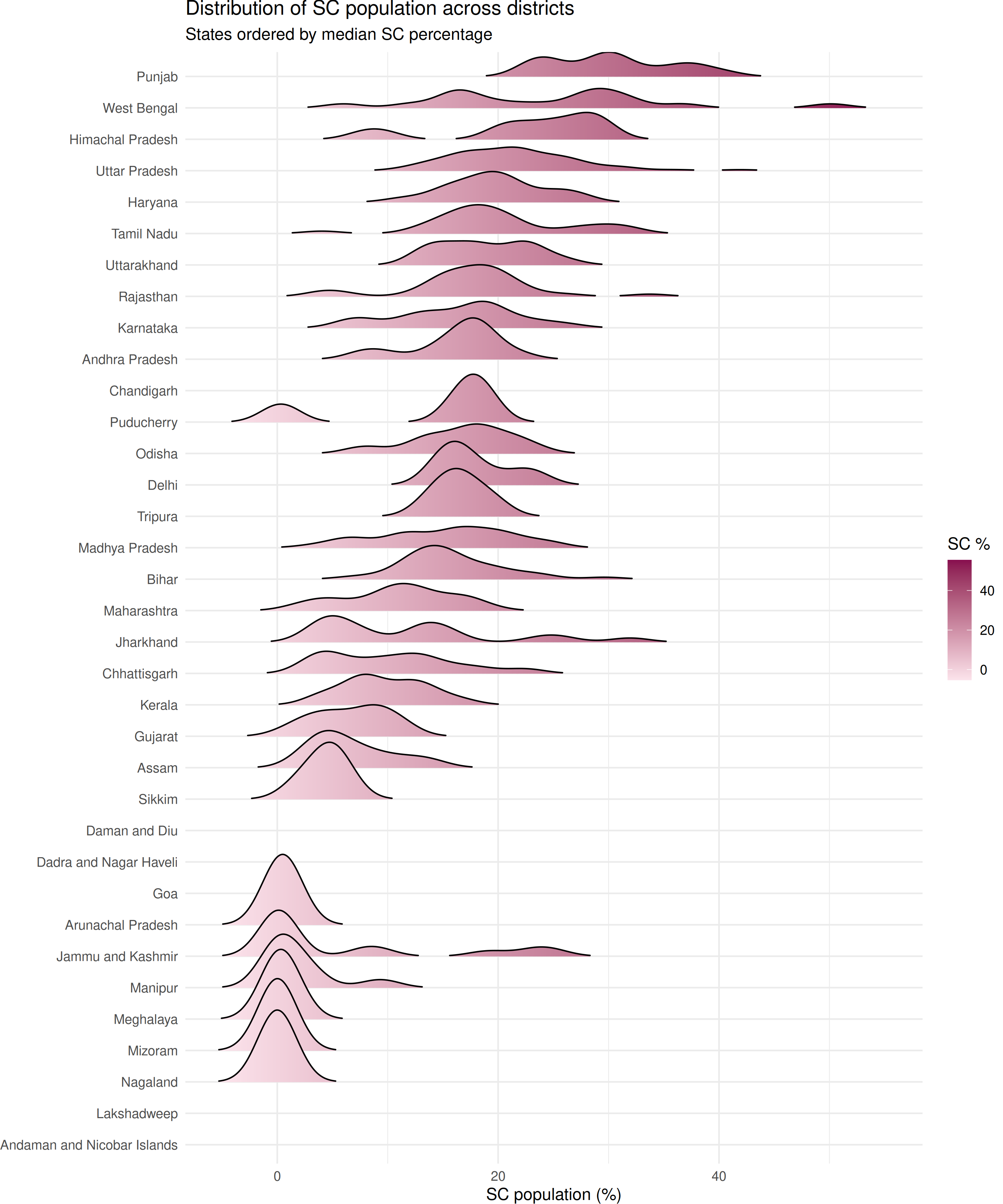

ST population distribution by state

state_order_st <- composition |>
  group_by(state_name_harmonized) |>
  summarise(median_st = median(st_pct, na.rm = TRUE)) |>
  arrange(median_st) |>
  pull(state_name_harmonized)

composition |>
  filter(state_name_harmonized %in% state_order_st) |>
  mutate(state_name_harmonized = factor(state_name_harmonized, levels = state_order_st)) |>
  ggplot(aes(x = st_pct, y = state_name_harmonized, fill = stat(x))) +
  geom_density_ridges_gradient(scale = 2, rel_min_height = 0.01) +
  scale_fill_gradient(low = "#e8f5e9", high = "#1b5e20", name = "ST %") +
  labs(
    x = "ST population (%)",
    y = NULL,
    title = "Distribution of ST population across districts",
    subtitle = "States ordered by median ST percentage"
  ) +
  theme_minimal() +
  theme(legend.position = "right")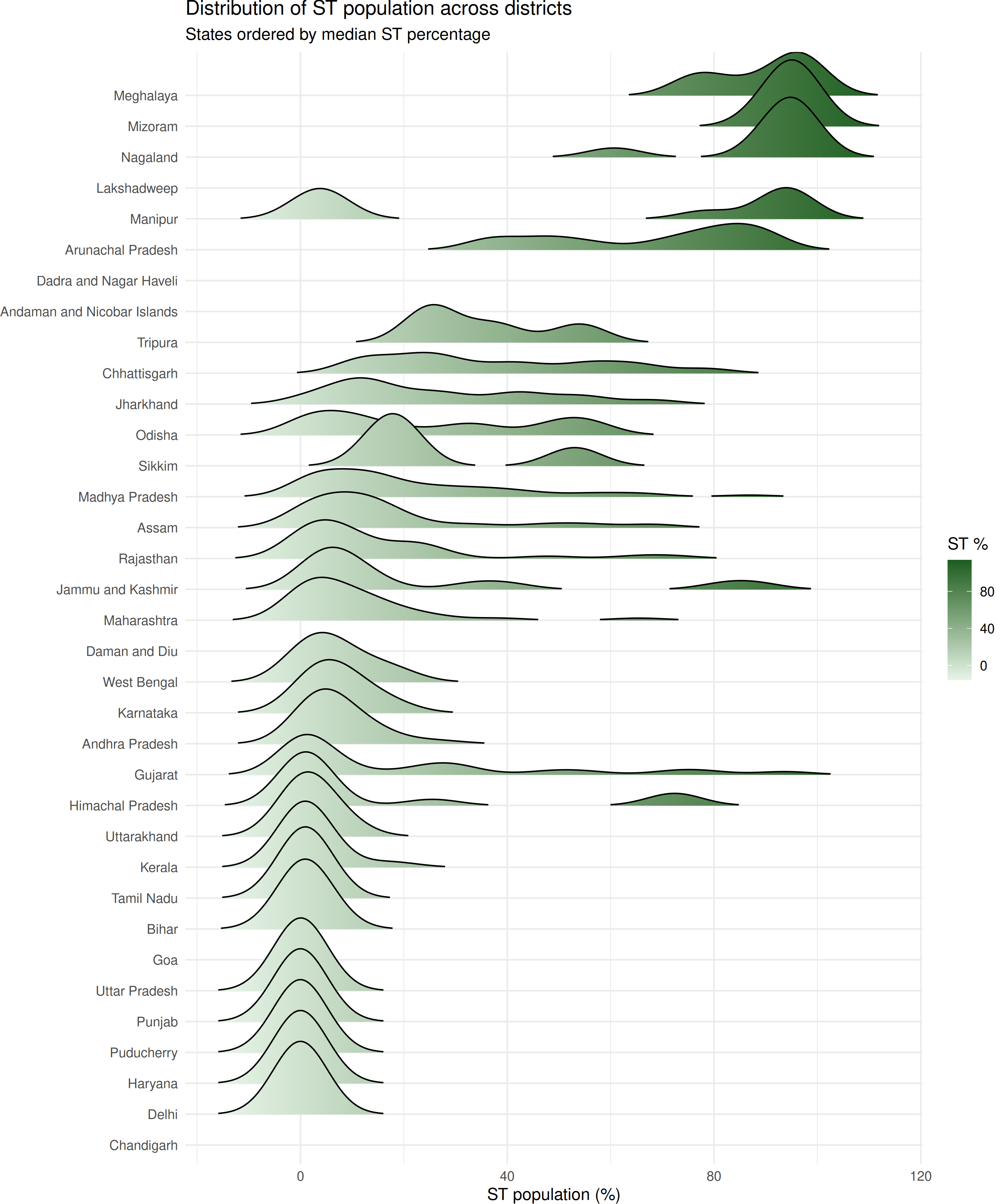

Linguistic diversity vs social composition

diversity <- census_2011_mother_tongue |>
  filter(language_level == "L1", district_code != "000", !grepl("Others", language_name)) |>
  group_by(state_name, district_code, area_name) |>
  mutate(proportion = total_persons / sum(total_persons)) |>
  summarise(
    effective_languages = 2^(-sum(proportion * log2(proportion), na.rm = TRUE)),
    .groups = "drop"
  )

diversity_composition <- composition |>
  mutate(district_code_chr = sprintf("%03d", district_code)) |>
  inner_join(
    diversity |> select(district_code, effective_languages),
    by = c("district_code_chr" = "district_code")
  )

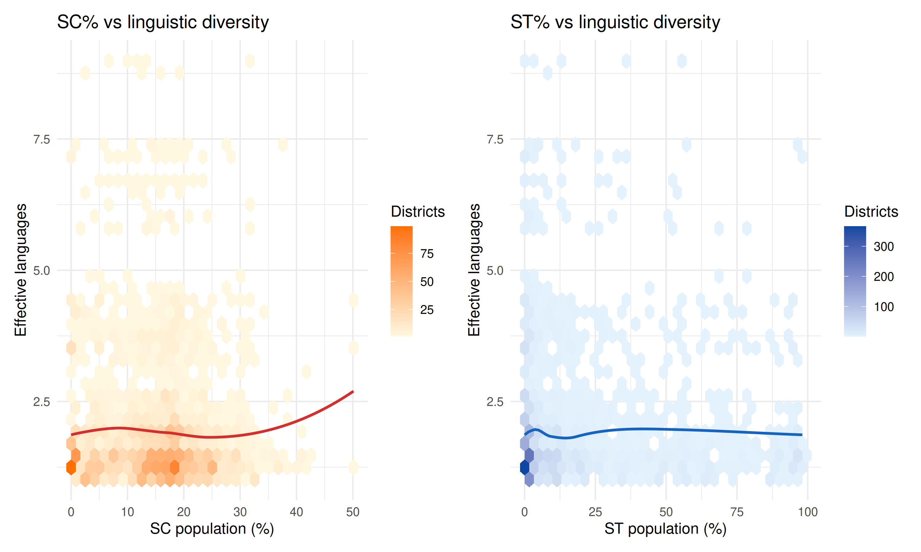
p1 <- ggplot(diversity_composition, aes(sc_pct, effective_languages)) +
  geom_hex(bins = 30) +
  geom_smooth(method = "loess", color = "#d32f2f", se = FALSE, linewidth = 1) +
  scale_fill_gradient(low = "#fff8e1", high = "#ff6f00", name = "Districts") +
  labs(
    x = "SC population (%)",
    y = "Effective languages",
    title = "SC% vs linguistic diversity"
  ) +
  theme_minimal()

p2 <- ggplot(diversity_composition, aes(st_pct, effective_languages)) +
  geom_hex(bins = 30) +
  geom_smooth(method = "loess", color = "#1565c0", se = FALSE, linewidth = 1) +
  scale_fill_gradient(low = "#e3f2fd", high = "#0d47a1", name = "Districts") +
  labs(
    x = "ST population (%)",
    y = "Effective languages",
    title = "ST% vs linguistic diversity"
  ) +
  theme_minimal()

p1 + p2